For the third edition of my Exploratory Data Analysis (EDA) series, I shall be exploring the human heart, computationally. The inspiration for this topic came from a quote in the recently released film The Man Who Knew Infinity:
“There are no proofs nor underlying laws that can determine the outcome of matters of the heart.”
— G.H. Hardy
Based on the real-life story of Srinivasa Ramanujan, the film takes us through the journey of this self-taught mathematical prodigy from Madras, India to Cambridge, England, where he formally develops mathematical proofs under the supervision of G.H. Hardy. Although I found it quite entertaining and quite enlightening on the life of Ramanujan, I was rather disappointed by the dissimilarity in physique between S. Ramanujan and Dev Patel (who played him, excellently), amongst other little things I later discovered were not so accurate. I think some of the minute inaccuracies were intentional or perhaps allowed for cinematic appeal. It is a brilliant film, nonetheless.
Now, I should note that this article discusses zero mathematics, in contrast to the film. The quote got me thinking about the human heart and I decided to computationally explore it—in linguistics, word translations, in published texts, and anatomy. My exploration here, as in previous EDAs utilises the Wolfram Language (WL) for its plethora of in-built functions. More improtantly, the WL gives direct access to a large database of curated data covering several areas of knowledge. This is very convenient—in combination with its computational power—for in-depth analysis such as this.
1. Semantics
Words
So... what is a heart? The DictionaryLookup function contains 92,518 words, which can only be searched for using a string pattern. However, WordData gives one access to 149,191 words and information on word properties such as definitions, phonetic form (IPA), WordNet ID, etc.
*As of 22 Nov 2016, on Mathematica 11.
1(Thread[WordData["heart", #] & /@ {"Definitions", "Synonyms"}] /. {a_, b_} :> {a, Last@b})/.2 {{word_, ps_, mean_} -> def_, syn_} :>3 {4 Row[{5 word, "[", Style[ps, Gray], "]: ",6 Style[mean <> "\t", Blue]7 }],8 Row[{9 def,10 If[Length[syn] > 0, Style[StringTemplate[" (``)"]@Row[syn, " | "],11 Lighter[Purple, .5]]]12 }]13 } // formGrid
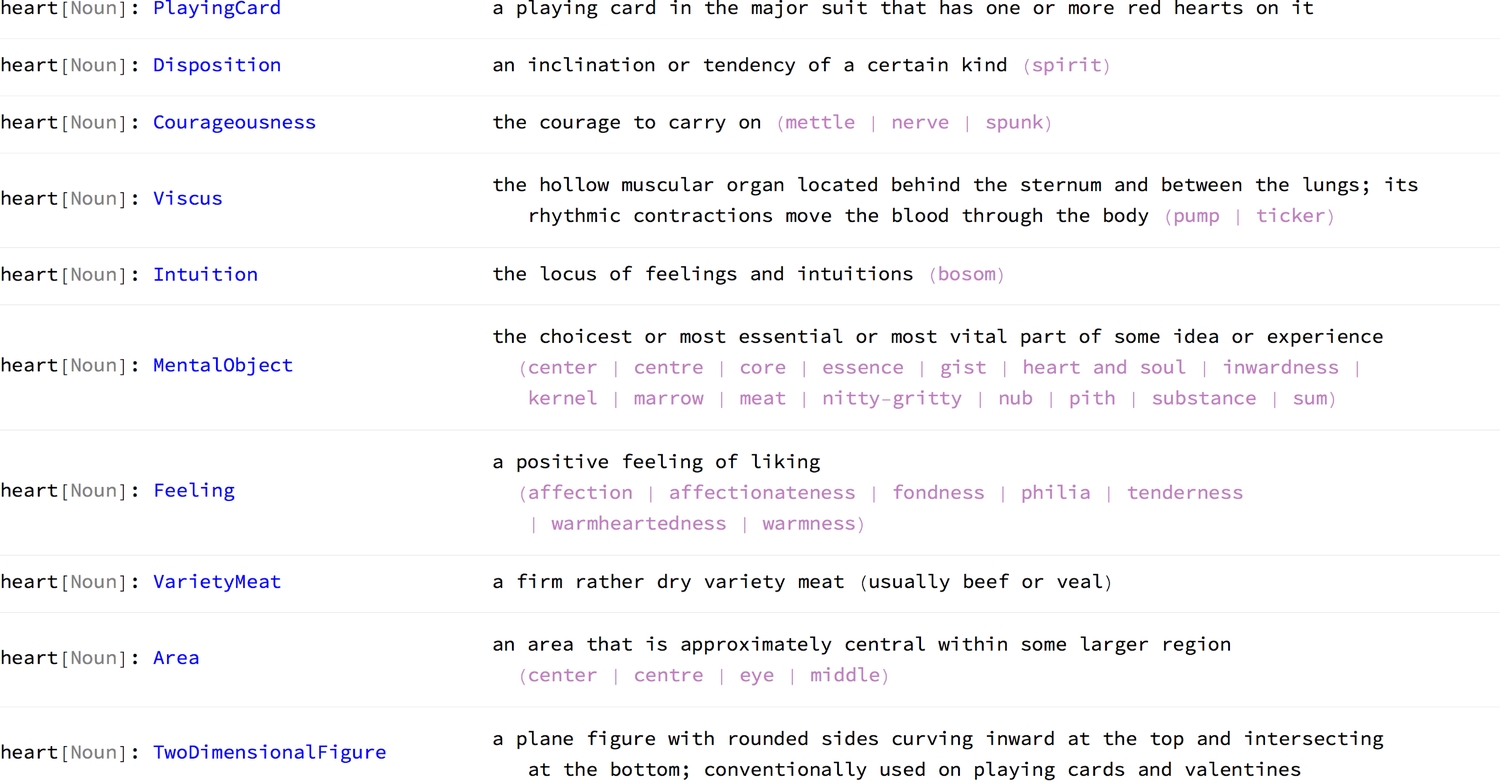
The definitions themselves offer ideas on the various paths one could take when exploring what the heart is. More importantly, they give insight into the present-day use of the word. I'm surprised to see that it is not recognised as a verb. The Internet, especially Social Media, has transformed the heart symbol into an icon that represents the act of liking or loving something. To better understand its nounal meanings, one can look into their individual linguistic properties. Out of the wide range of possible queries, I have selected the concept weight of each definition, its broader and narrower terms, and an example sentence.
1((# -> Association[WordData["heart", #] /.2 ({_, _, l_} -> s__) :> Style[l, Blue] ->3 Shallow[Text@OutputForm@s, {6, 3}]]) & /@4 {"BroaderTerms", "ConceptWeight", "Examples", "NarrowerTerms"}) /.5 {} -> "-" // Association // Transpose // Dataset

When one uses the word heart, one is most likely referring to the "wildly thumping organ" or the "feeling," because they have the highest concept weights (which the documentation says is a "rough estimate of semantic importance"). What's more, heart can be interpreted as a word or an anatomical structure.
Interpreter[#]["heart"] & /@ {"Word", "AnatomicalStructure"}

The Wolfram Language offers instant access to quite an extensive volume of information about the real world. The several domains of knowledge covered are represented by Entities. As your read on you come across more entities, with orange rounded borders and a light orange background. For now, we'll focus on the linguistic entity. We can learn more about a word by exploring its EntityProperties—shown below are some more properties not covered by WordData. I was impressed to see the <3 (or ♥︎) texting form.
1ReplaceAll[(CommonName[#] <> ": " ->2Entity["Word", "heart"][#] & /@ (EntityProperty["Word", #] &/@3 {"CompoundWords", "LanguageOrigin",4 "NYTCrosswordPuzzleClues", "Phrase",5 "Rhymes", "TextAbbreviations"})),6 (a_ -> b___) -> {a, Short[b, 2]}] // formGrid

Anatomical definition
We can find out the anatomical function of the heart quite easily, as well as its Wikipedia definition.
1(* define an anatomical entity - the heart *)2heart = Entity["AnatomicalStructure", "Heart"];3(* find out what it does *)4heart[EntityProperty["AnatomicalStructure", "Function"]]

1(* article summary *)2wikiPlainText = WikipediaData["Heart", "SummaryPlaintext"];3(* take first two sentences of each paragraph *)4StringRiffle[StringRiffle /@ (TextSentences[#][[;; 2]] &/@5StringSplit[wikiPlainText, "\n"]), ".. \n\n"]

2. Languages and translation
I found that one of the properties obtainable for the entity of an anatomical structure is its Latin name. However, when I compared the returned result, cor, to the WL translation there was no match. A quick check on Google Translate shows that both results are indeed Latin for heart.
{heart["LatinName"], WordTranslation["heart", "Latin"]} gives {{"cor"}, {"viscus", "pectus", "pectoris"}}.
Unfortunately the documentation for WordTranslation function does not say anything regarding its sources. Nonetheless, let's translate heart to all languages available:
transl = KeySort@WordTranslation["heart", "English" -> All];
Short[%, 3]

We get 182 translations! Some languages have more than one word for heart. Some languages probably share the same word(s) for heart, perhaps due to their proximity in classification or geography, lexical similarity or for some other reason. It appears that all translations to German begin with capital letters. I do not know if these are like proper nouns in English, but I will convert all words to lowercase.
Group by word
1sharedTransl = GroupBy[Flatten[Thread /@ Normal[transl]] /.2 (e_Entity -> w_String) :> e -> {ToLowerCase@w}, Extract[Last@#, 1] & -> First];3(* select words shared between more than one language *)4formGrid[KeySort@KeySelect[GroupBy[Normal@%, Length[Last@#] &], # > 1 &], "BoldLeft"]

Now, we learn that "jantung" is the most shared word, for heart, amongst different languages (Batak, Bugis, Indonesian, Javanese, Madura and Malay) around the world.
For each translation, we can also find the country with the highest number of speakers of that language. To do this, we'll relate each word to its language, and each language to the country with the highest number of speakers.
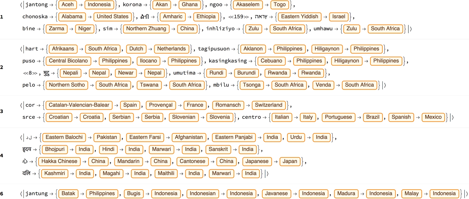
We discover that although the word "jantung" may come up in six different languages, these languages are spoken (mostly) by people living in only two countries--Indonesia and the Philippines. Now, we'll group according to the countries. Our objective here is to find the country with the most number of distinct words or language translations for heart.
Group by country
Detailed information about a lot of languages spoken around the globe is also accessible from the WL. Our goal here is to associate each language (and its translation) to the country which has the largest number of people speaking that language. For a few languages, the countries are not stated and so we'll delete such cases. Similarly, the language Papiamentu is found to be spoken mostly in the Netherlands Antilles, which the Wolfram Database does not recognise as a country. I have replaced it with a country entity of the Netherlands. Now, we'll count the number of translations found in each country and group the countries by this number.
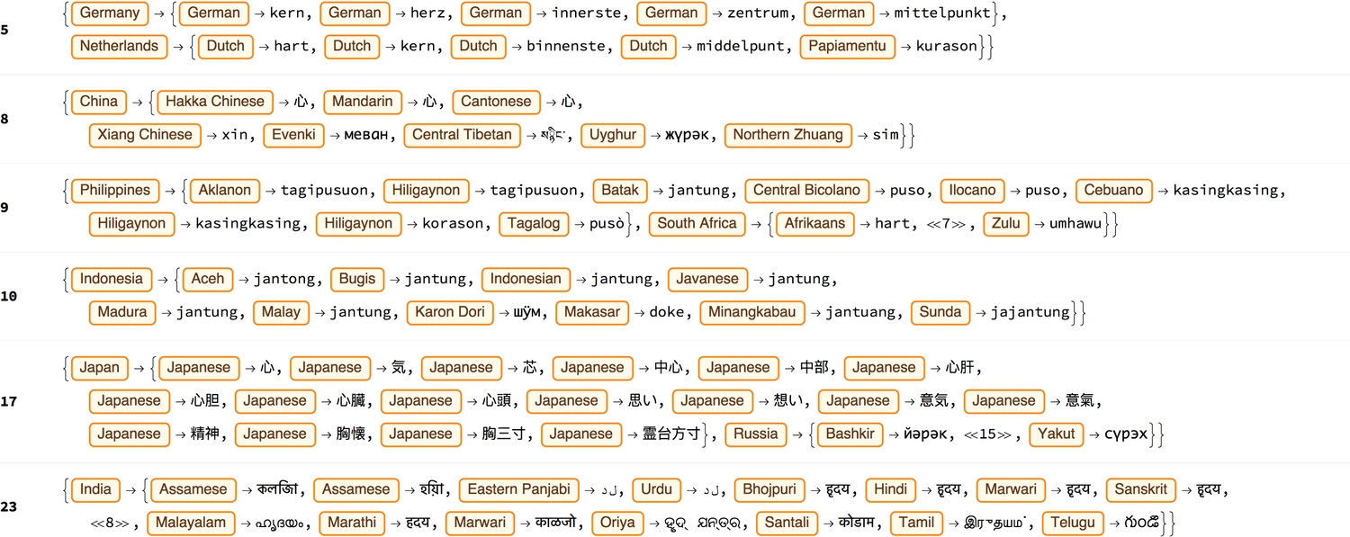
India leads with 23 translations of the word heart, followed by Japan and Russia, with 17. Note the similarity between words in Indonesian languages (starting with 'ja(n)' and ending with '(u)ng'). Also, do certain words begin with a capital letter in German? I had to amend my code to change all translations to lowercase. Please comment below if you know German. :)
Country—language—word interrelationship
To better understand the interplay between countries, languages and words, I decided to combine everything into a single graph, converting all words to lowercase. We should expect to see connections between countries that share borders, are near each other or have had historical relations (e.g. colonialism, war, migration, etc.). The graph turned out to be more interesting than I imagined.
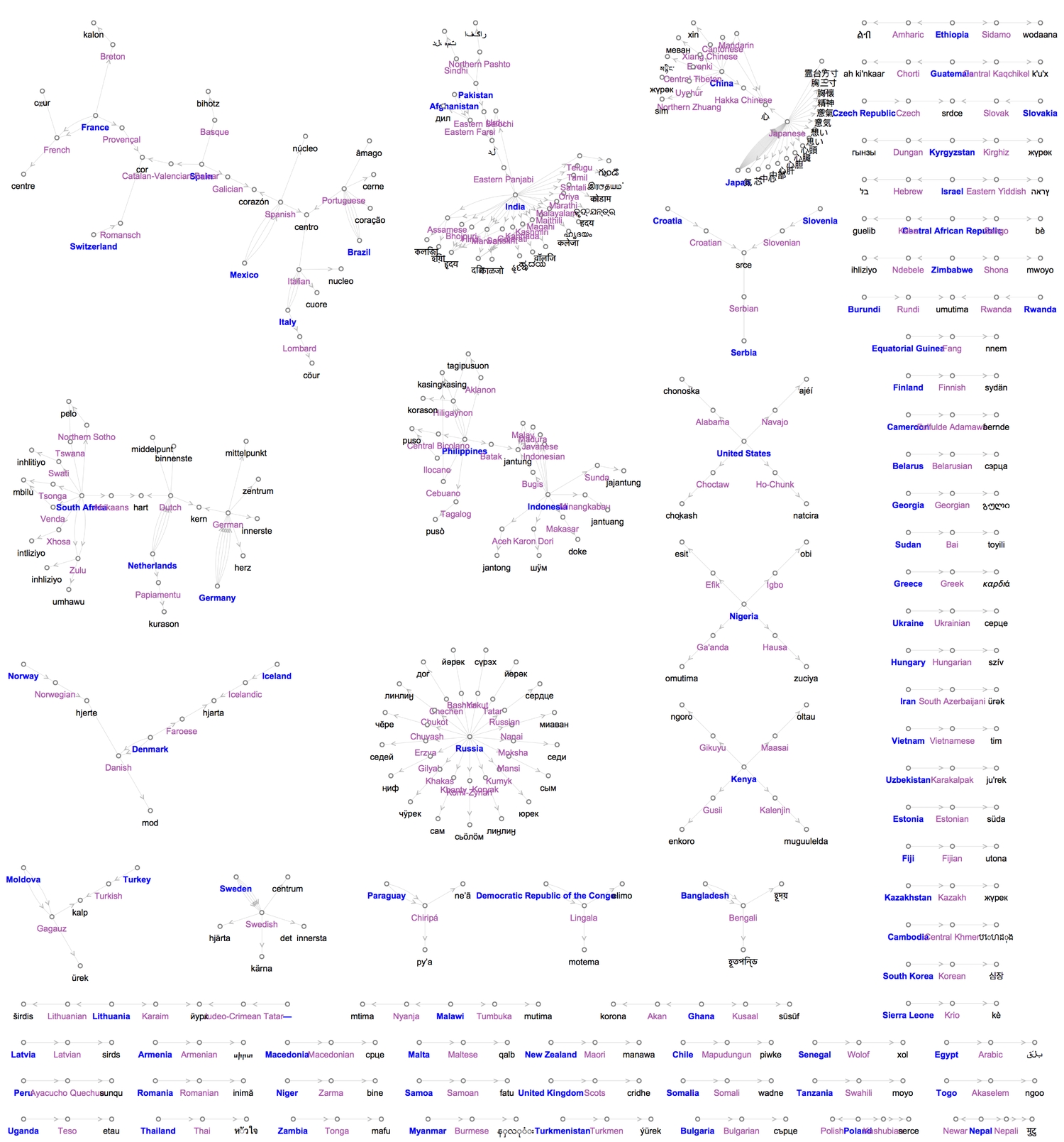
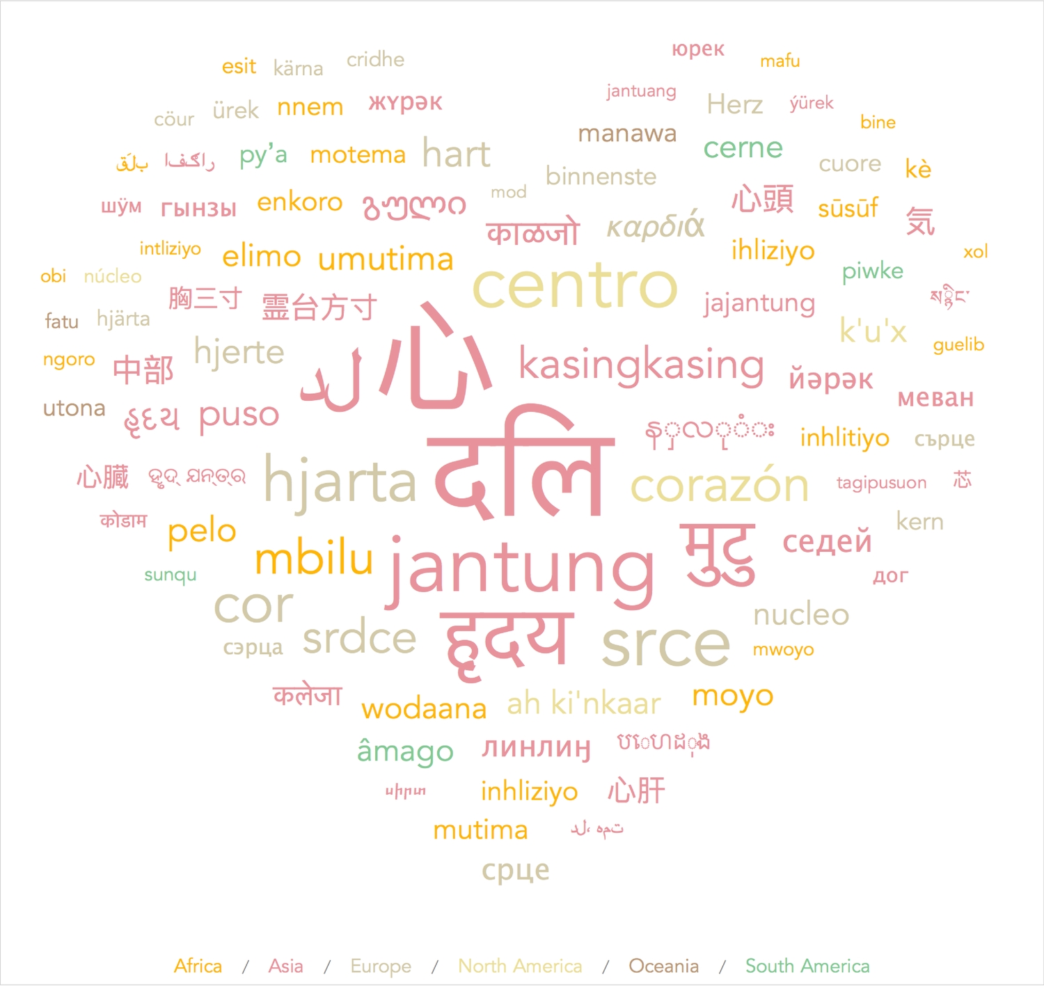
The graph will be different if were to connect each country with all languages spoken in it. We can also colour each word translation according to its continent because we already have its country. To do this we'll create a Wordcloud. For some reason, only up to a hundred words are shown.
Language distances
Earlier we grouped the words by the countries with the highest number of speakers of that language. From this new grouping, we'll select the words that are spoken in two or more countries.

For each word, we can then find the geographical distance between the two or more locations in which one may hear the word being said. The distances are calculated from the centre of one country to that of the other. Let's call this the heart-lang distance.
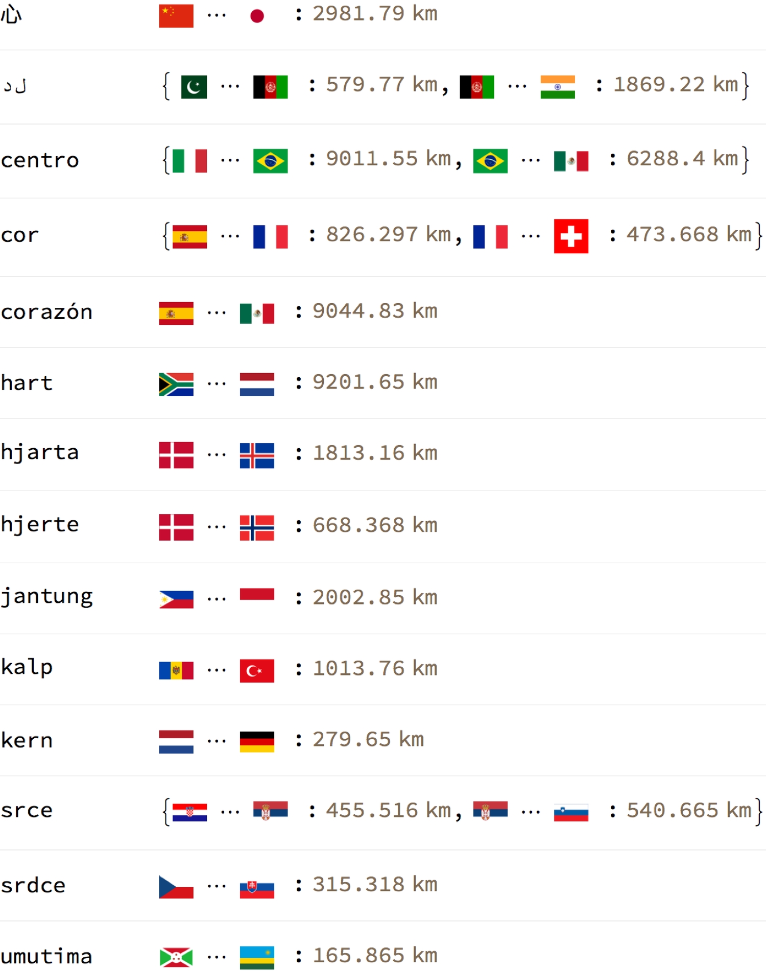
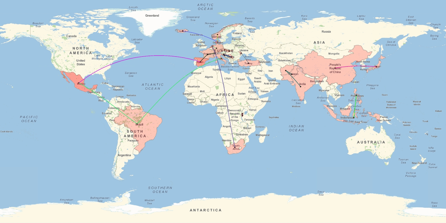
'Hart' has the greatest heart-lang distance (~ 9200 km) from South Africa to the Netherlands while 'umutima' has the smallest (~165 km) from Burundi to neighbouring Rwanda. To better visualise the heart-lang distances we plot them all on a single map. The map shows most of the countries which share the same word for heart, joined by a path line, to be near each other, or even be sharing borders. I think the few anomalies owe to the olden colonial days. I wonder what else one can learn about the world by looking at relationships between languages and where they are spoken.
Transliteration
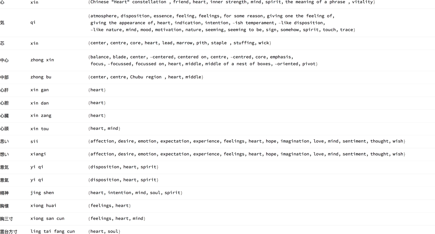
Transliteration is also possible in the WL. Let's take a look at the Japanese words, their transliterations and translations back to English.
1Transliterate[{"心", "気", "芯", "中心", "中部", "心肝", "心胆", "心臓", "心頭",2"思い", "想い", "意気", "意氣", "精神", "胸懐", "胸三寸", "霊台方寸"}]

1{#, Transliterate[#], WordTranslation[#, Entity["Language", "Japanese"] ->2Entity["Language", "English"]]} & /@3 {"心", "気", "芯", "中心", "中部", "心肝", "心胆", "心臓", "心頭", "思い",4 "想い", "意気", "意氣", "精神", "胸懐", "胸三寸", "霊台方寸"}5 // Style[formGrid[#], 12] &
3. Heartwords
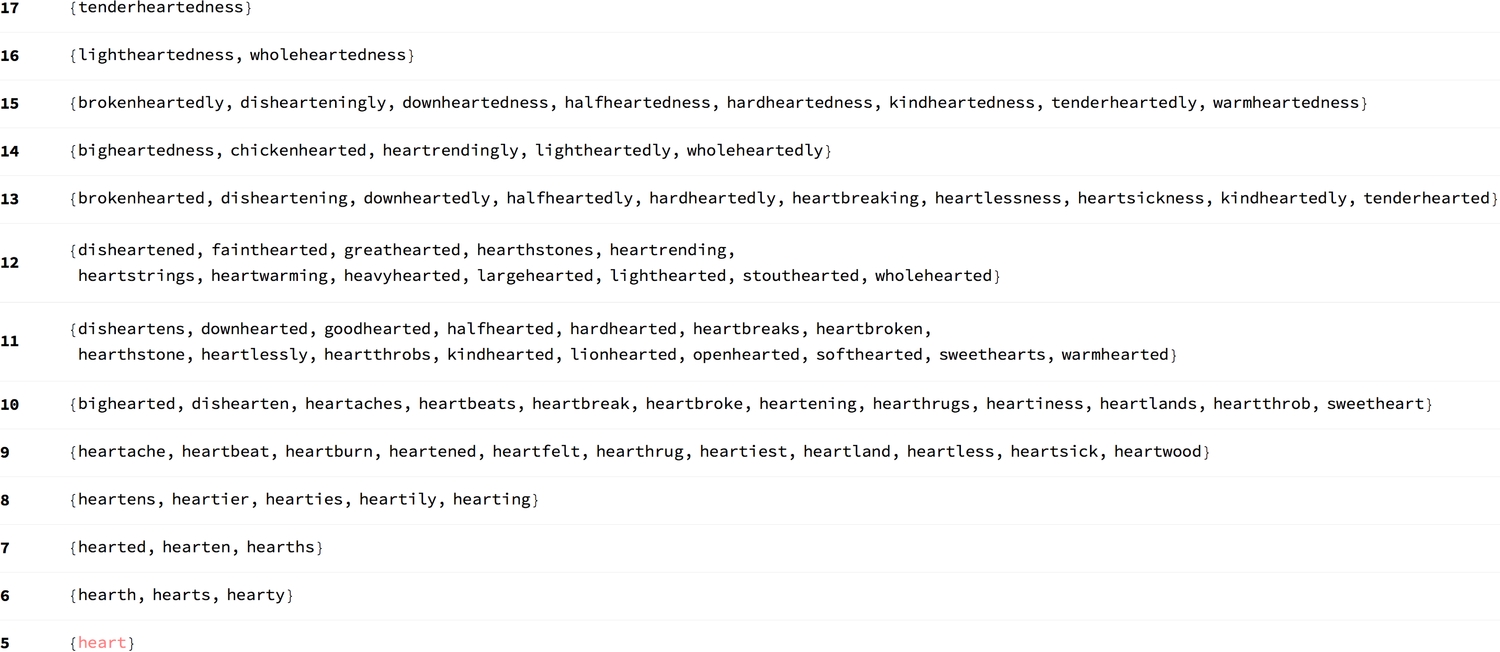
Back to linguistics... As I explored this topic of the heart, I slowly gleaned the essence of words regarding matters of the heart. Particularly, in the description of a person's character. 89 English language words contain 'heart' in them, and 21 of those words adjectivally end with 'hearted.' Therefore, at least in the English language, a lot is conveyed, metaphorically, with the heart. For all words that contain 'hearted,' the letters that come before it are highlighted in blue below.
1(* adjectives containing 'hearted' * heartedWords2DictionaryLookup["*hearted*"];3heartedWordsHighlighted = StringReplace[#, bfHeart : __ ~~ "heart" ~~ rest__ :>4 "\!\(\*StyleBox[\"" <> bfHeart <> "\",FontColor->RGBColor[0,0,1]]\)"5 <> "heart" <> rest] &/@ heartedWords;6Grid[Partition[myFrame[#] & /@ Sort@heartedWordsHighlighted, 5], Alignment -> Left]

1(* gather all --people-- words that have a 'heart' *)2heartWords = DictionaryLookup["*heart*"];3formGrid[KeySortBy[GroupBy[heartWords, StringLength], Minus] /.4 heartStyleRule, "BoldLeft"]
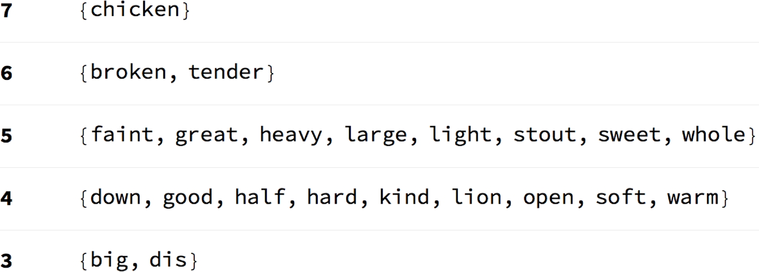
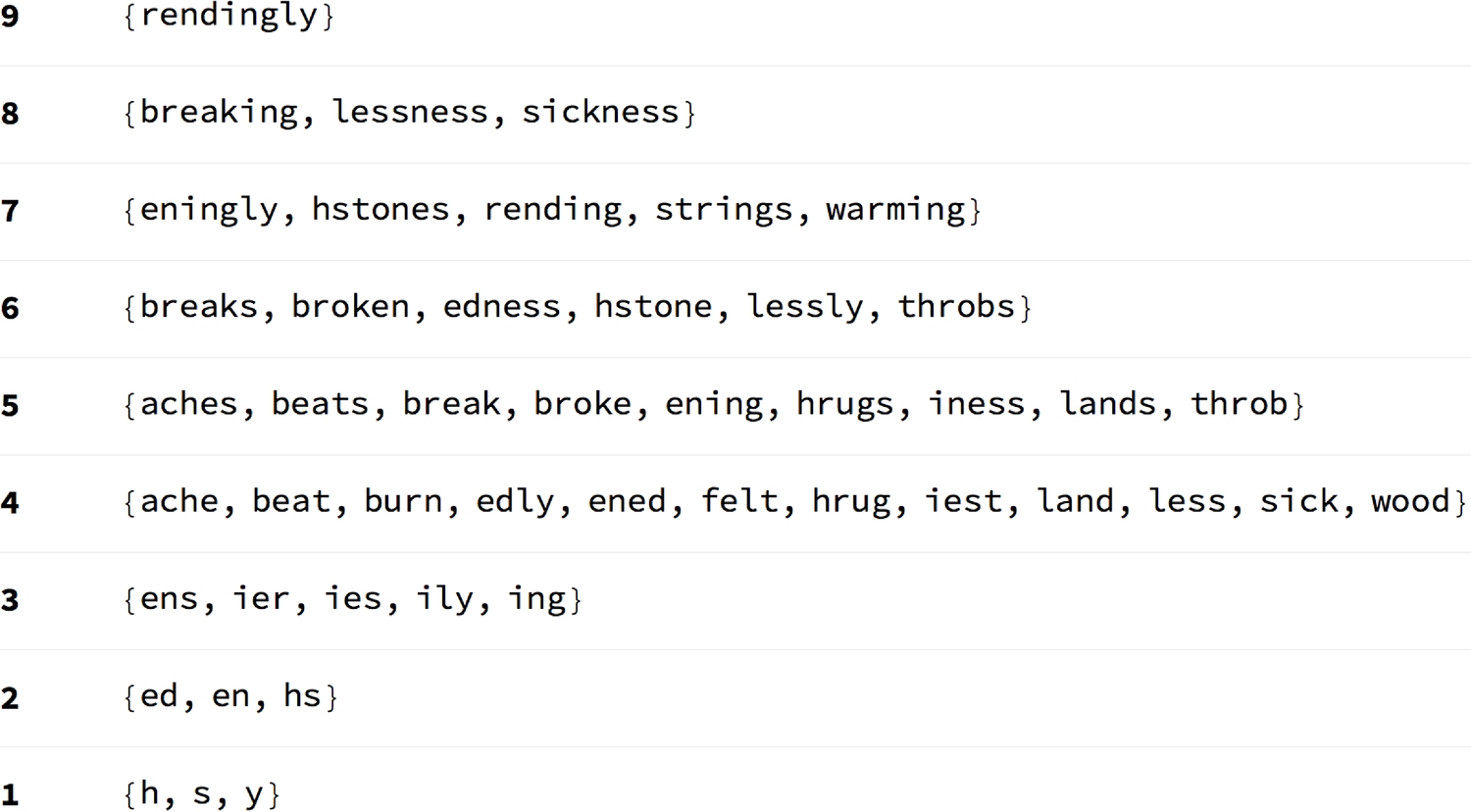
Let's find the longest words before and after 'heart':
1longBfHeart = First@SequenceAlignment[#, "heart", Method -> "Local", IgnoreCase -> True] & /@ heartWords;2longBfHeart = DeleteCases[DeleteDuplicates@longBfHeart, "heart"];3formGrid[Sort /@ KeySortBy[GroupBy[longBfHeart[[;; , 1]], StringLength], Minus], "BoldLeft"]45longAfHeart = Last@SequenceAlignment[#, "heart", Method -> "Local", IgnoreCase -> True] & /@ heartWords;6longAfHeart = DeleteCases[DeleteDuplicates@longAfHeart, "heart"];7formGrid[Sort /@ KeySortBy[GroupBy[longAfHeart[[;; , 1]], StringLength], Minus], "BoldLeft"]
Clustering
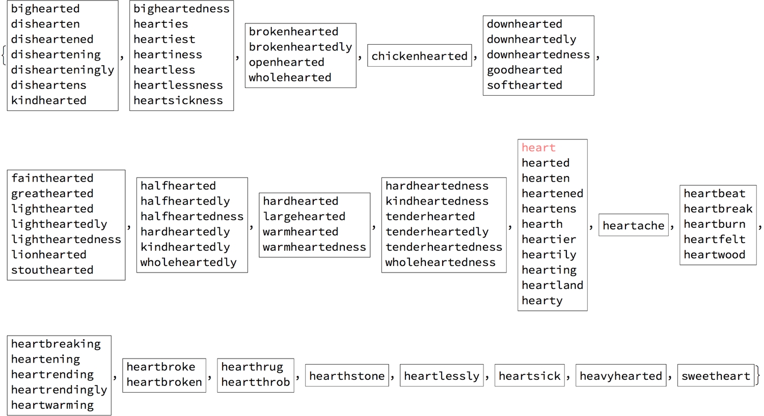
We can group the words by their Levenshtein (or edit) distances, i.e., the number edits required to transform one string to another.
1(* pluralise all *) myPluralize[word_] := Check[Pluralize@word, Nothing];2(* remove plurals *) withoutPlurals = Quiet@Complement[heartWords, myPluralize /@ heartWords];34(* cluster into 20 groups *)5heartClusters[num_] := Framed[Column@If[Length[#] > 15, {Multicolumn[#, 2]}, #]] & /@6 FindClusters[withoutPlurals, num,7 Method -> "KMedoids",DistanceFunction -> EditDistance, PerformanceGoal -> "Quality"] /. heartStyleRule;8heartClusters[20]
We can also cluster the words into a dendrogram.
1Dendrogram[withoutPlurals -> (Rotate[#, Pi/2] &/@2withoutPlurals),3Top, ClusterDissimilarityFunction -> "Complete", DistanceFunction -> EditDistance, ImageSize -> 1000] /. heartStyleRule
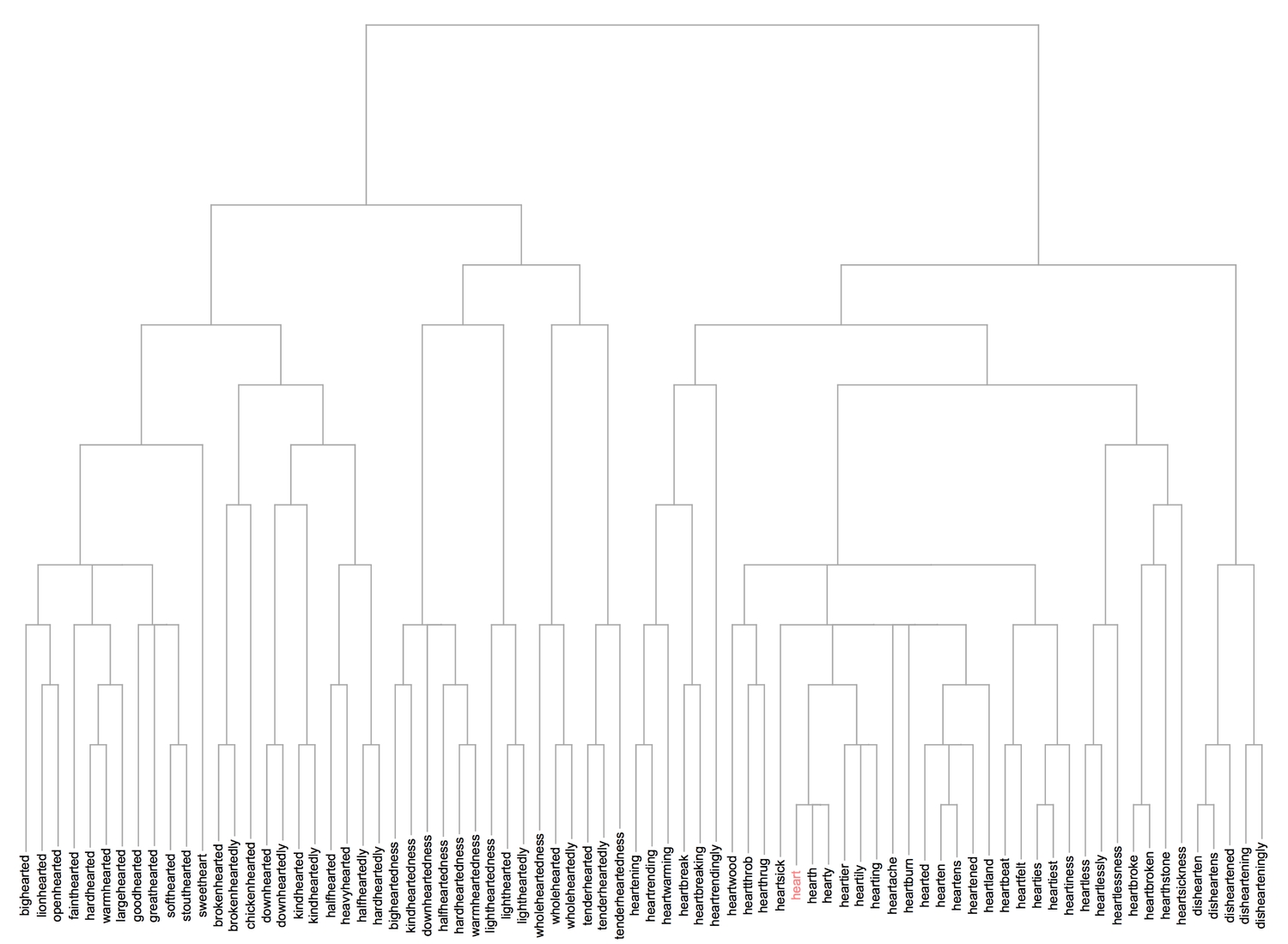
One can specify the desired cluster dissimilarity function, either from the list of inbuilt functions or a custom one. I have used the inbuilt "Complete" function which utilises the largest dissimilarity between clusters to plot the dendrogram. The clustering shown in the dendrogram appears to be more precise than the framed clusters of words. One more visualisation method is the clustering tree.
1ct = ClusteringTree[withoutPlurals -> (Style[#, 9] & /@ withoutPlurals /. heartStyleRule), ClusterDissimilarityFunction -> "Complete", PerformanceGoal -> "Quality", GraphLayout -> "RadialDrawing"];23(* highlight the shortest path from the root vertex to 'heart' *)4myFrame@HighlightGraph[ct, PathGraph[FindShortestPath[ct, 1, 103]], EdgeShapeFunction -> ({Opacity[1], Pink, Line[#1]} &), ImageSize -> 1000]
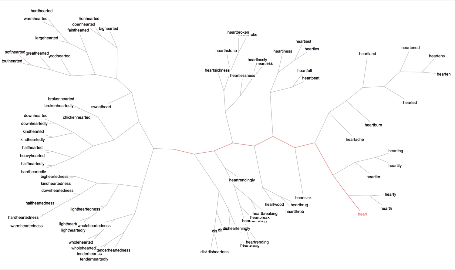
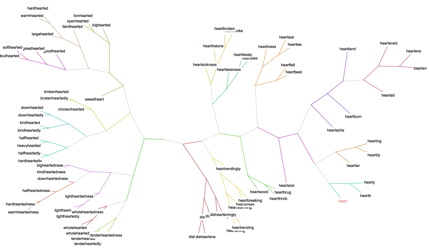
The tree essentially is a graph, and therefore one can attempt to find communities within the graph using the FindGraphCommunities function. Here's a good paper that gives a detailed explanation of graph communities and examples.
1(* use spectral-based clustering to partition graph *)2HighlightGraph[ct, Map[Subgraph[ct, #] &,3 FindGraphCommunities[ct, Method -> "Spectral"]],4 GraphHighlightStyle -> "DehighlightGray", ImageSize -> 1000]
4. Word relations
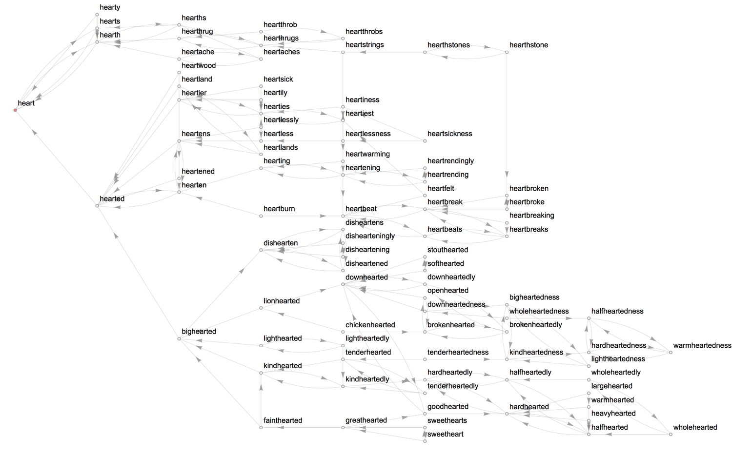
Having examined heartwords (words that contain 'heart') in the previous section, we'll examine the characteristic relationships between them. We need a graph-plotting function to visualise the connections established by the linguistic properties we'll be looking at.
1formRelationGraph[propertyTest_, wordList_List, opts__: (DirectedEdges -> True)] :=2 Block[{graph},3 graph = RelationGraph[propertyTest, wordList];4 ReverseGraph @ Graph[EdgeList[graph] /. {(v__ \[DirectedEdge] v__) -> Nothing, (y_ <-> y_) -> Nothing, (z_ -> z_) -> Nothing, heartStyleRule}, opts,5 VertexLabels -> "Name", VertexSize -> .3, VertexStyle -> Directive[White, EdgeForm[Gray]],6 EdgeStyle -> Directive[Thickness[.00025], Gray], EdgeShapeFunction -> GraphElementData["Arrow", "ArrowSize" -> 0.01],78 GraphLayout -> {"VertexLayout" -> "SpringElectricalEmbedding", "PackingLayout" -> "ClosestPacking"}, ImageSize -> 1000]9 ];
Parts of speech
The first property we'll look at is part-of-speech. The following function tests two strings for sameness in (any) part-of-speech, returning a Boolean result.
1samePartOfSpeechQ[word1_String, word2_String] := AnyTrue[Table[MemberQ[#1, i], {i, #2}], TrueQ] &@@2 {PartOfSpeech[word1] /. Missing[_] -> {}, PartOfSpeech[word2] /. Missing[_] -> {}}
Now we can form a relation graph for part-of-speech. I have added extra steps to remove self-loops and to highlight and label the different graph communities (parts of speech).
1(* relation graph *)2gPoS = formRelationGraph[samePartOfSpeechQ, heartWords,3VertexSize -> 0.2, PlotTheme -> "Monochrome",4EdgeStyle -> Directive[Thickness[.00025], Gray],5EdgeShapeFunction -> Automatic,6GraphLayout -> {"VertexLayout" -> "SpringElectricalEmbedding", "PackingLayout" -> "ClosestPacking"}];
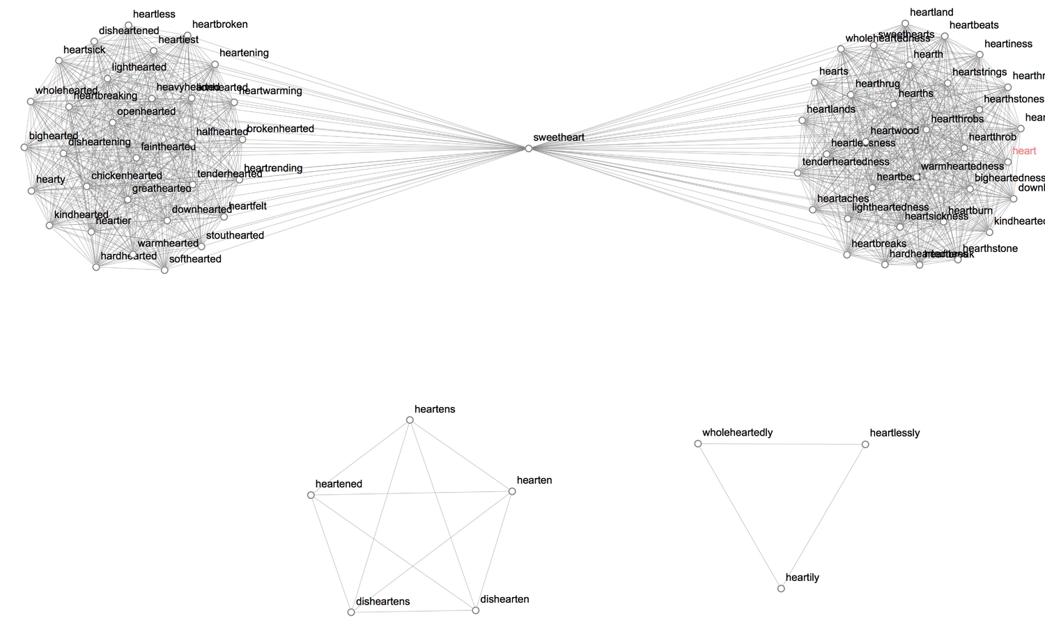
Let's highlight communities latent in the graph.
1(* highlight and label communities *)2CommunityGraphPlot[HighlightGraph[gPoS, Map[Subgraph[gPoS, #] &,3 FindGraphCommunities[gPoS, Method -> "Hierarchical"]], GraphHighlightStyle -> "DehighlightGray", ImagePadding -> 20],4 CommunityLabels -> (Style[#, 15, Blue] & /@ {"Nouns", "Adjectives", "Verbs", "Adverbs"})]
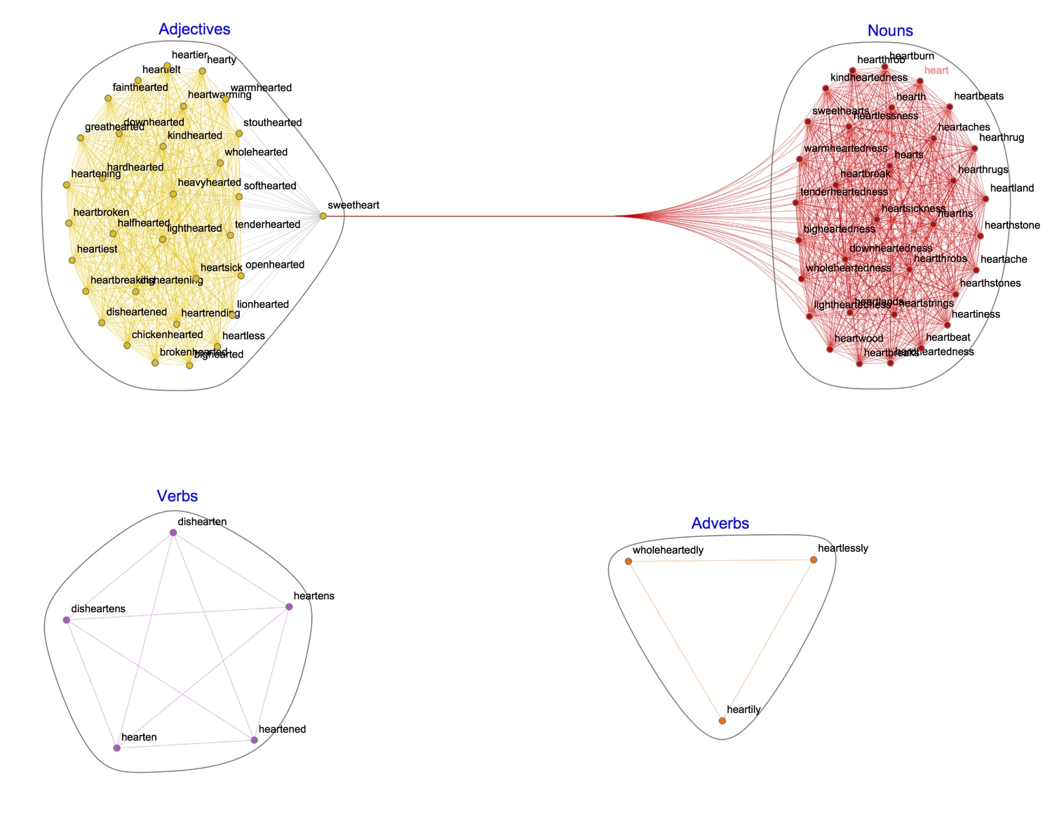
Each word is linked to every other word with which it shares a part-of-speech. Interestingly, the WL dictionary class "sweetheart" as a noun and an adjective.
String Patterns
WL, functions which end with the letter Q ask if a condition is satisfied. For example, ListQ[{1, 2, 3}] asks if {1, 2, 3} is a list, and returns a boolean result (True in this case). By evaluating Length@Names["*Q"] we discover that there are, as of Mathematica 11, 166 functions ending with Q.
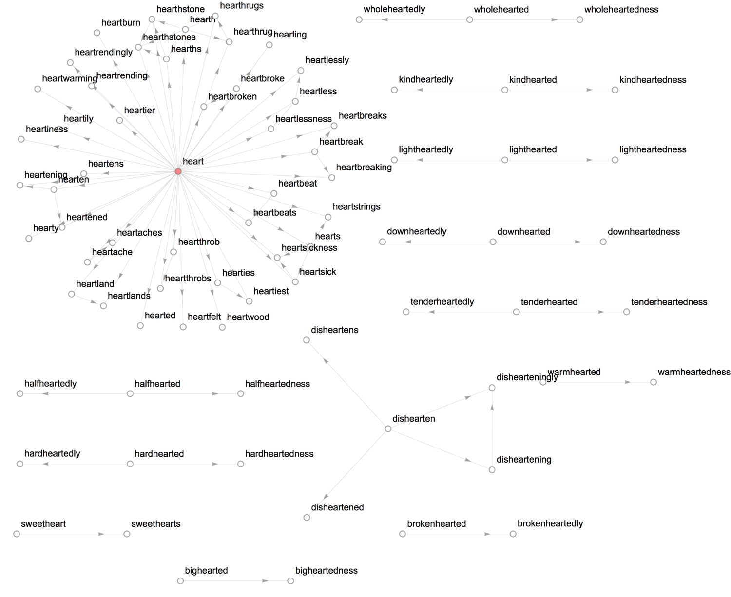
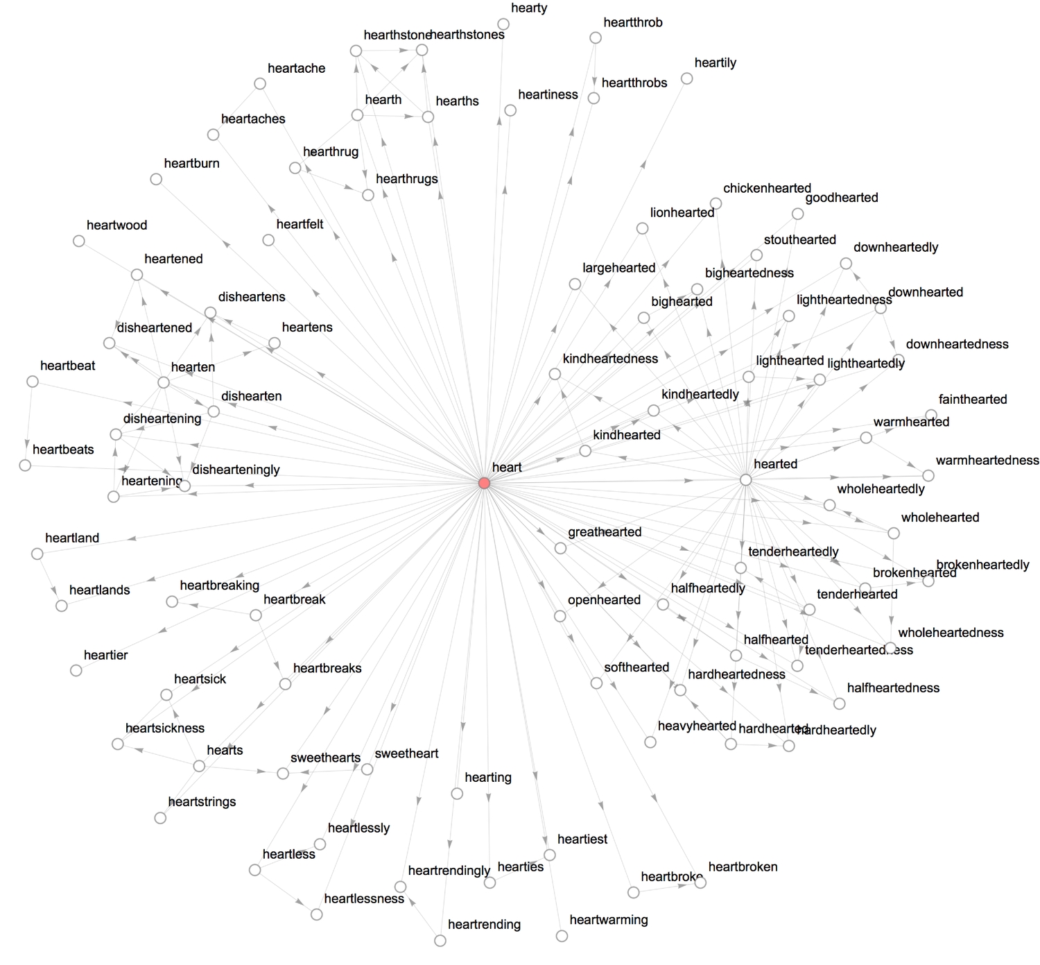
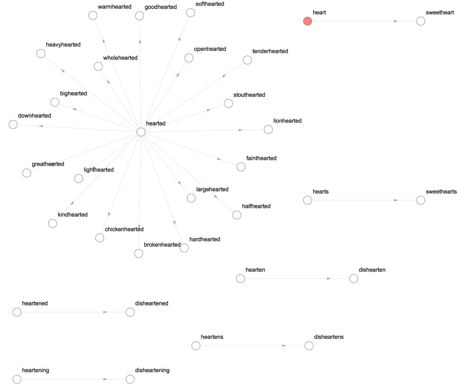
Our interest here is to form relationships between words that satisfy a few string-related conditions.
- StringContainsQ: If string
ucontains stringv, then form a directed edge betweenuandv.
1formRelationGraph[StringContainsQ, heartWords, VertexSize -> .2, ImageSize -> 800]
- StringStartsQ: If string
ucontains stringv, then form a directed edge betweenuandv.
1formRelationGraph[StringStartsQ, heartWords, VertexSize -> .2, ImageSize -> 800]
- Nearest heartword: Form a directed edge between each string and its three "nearest" strings.
1formRelationGraph[#1 =!= #2 && MemberQ[Nearest[heartWords, #2, 3, DistanceFunction -> EditDistance], #1] &, heartWords,2GraphLayout -> {"LayeredEmbedding", LayerSizeFunction -> (3 &),3 "RootVertex" -> "heart", "LeafDistance" -> .5, "Orientation" -> Left}, VertexSize -> 0.2, ImageSize -> 1000]
- StringEndsQ: If string
uends with stringv, then form a directed edge betweenuandv.
1formRelationGraph[StringEndsQ, heartWords, VertexSize -> .2, ImageSize -> 800]
5. Word frequencies
The final aspect of natural language we'll look at is the frequency of words in typical English published text, using the WordFrequencyData.
In English text
Find the total word frequency of the word 'heart' between 1700 and 2015, ignoring letter cases:
WordFrequencyData["heart", "Total", {1700, 2015}]
0.00020518
and in a permutation of letter cases, in descending order:
Reverse@Sort@WordFrequencyData["heart", "CaseVariants", {1700, 2015}]

The sum of the frequencies of distinct cases should equal the total for when cases are ignored (i.e., IgnoreCase -> True)
Plus @@ Values@%
0.000205184
For different parts of speech:
Reverse@Sort@WordFrequencyData["heart", "PartOfSpeechVariants"]

Find the ratio between the frequency of the word 'heart' to 'mind':
Divide @@ (WordFrequencyData[#, "Total", {1700, 2015}] & /@ {"heart", "mind"})
0.71481
This means that 'heart' has historically been used less than 'mind', in English texts. But what has the trend been like over the past centuries? (1700 was a very long time ago, so I've taken the moving average of the timeseries using a step of a decade.)
1plotOPts = {ImageSize -> 400, PlotStyle -> ColorData[64, "ColorList"]};2plotOPts = {ImageSize -> 400, PlotStyle -> ColorData[64, "ColorList"]};
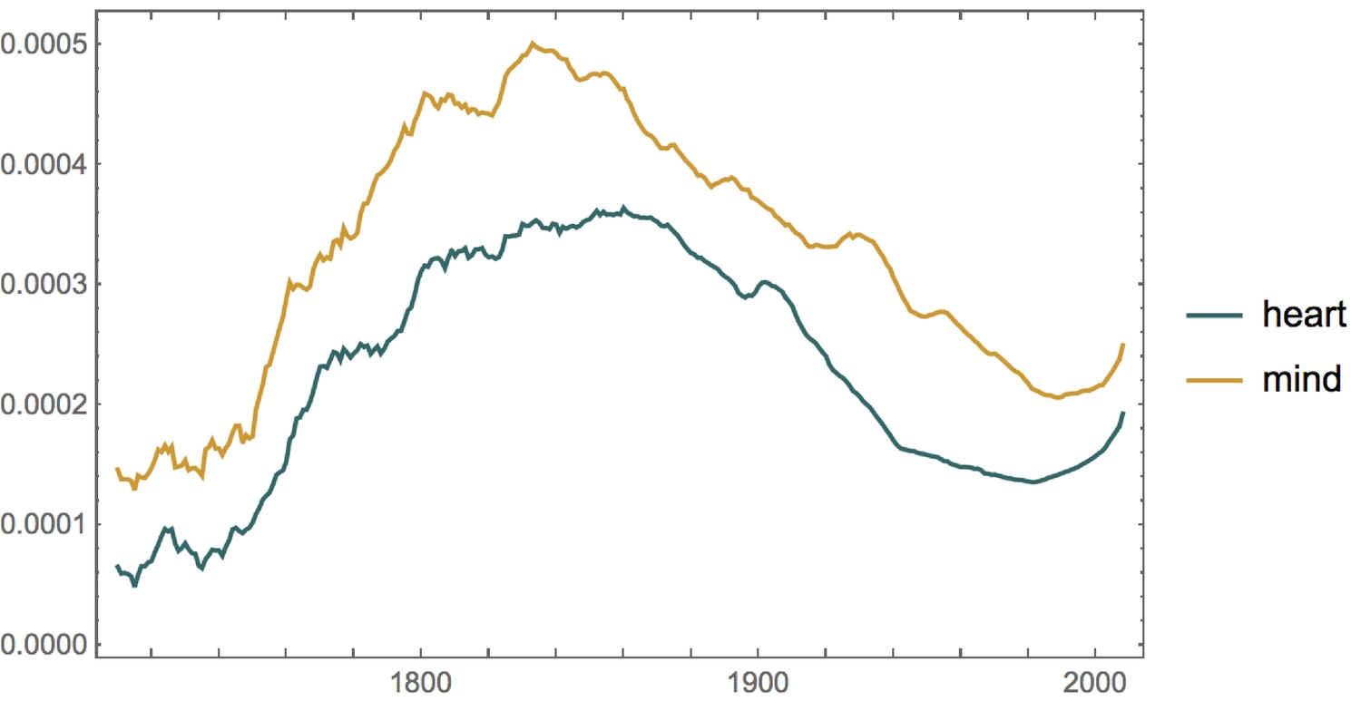
There seems to be a correlation between the use of the words 'heart' and 'mind', and the usage of both words (in English texts) is on the rise. One can access some APIs directly from the WL. One such API is the OpenLibrary. Using this API, we'll access the initial publish date of up to a thousand books, containing the words 'heart' and 'mind'.
1(* connect to OpenLibrary API *) openlibrary = ServiceConnect["OpenLibrary"];2(* heart and mind titles *)3{heartBookTitles, mindBookTitles} = openlibrary["BookSearch", {"Title" -> #, MaxItems -> 1000}] & /@ {"Heart", "Mind"};4(* publish dates *)5{heartPubDates, mindPubDates} = Cases[Normal[#[;; , "FirstPublishYear"]], _DateObject] & /@ {heartBookTitles, mindBookTitles};
The following function will allow us to automatically compare the historical word frequencies of two or more words. The function also uses a decade-long moving average step of the results.
1(* let's compare the word freqs. of two words *)2compareTwoCurves[words_List, opts__: {}] := Module[{f, l}, {f, l} = #[words] & /@ {First, Last};3DateListPlot[MovingAverage[WordFrequencyData[#, "TimeSeries", {1700, 2015}],4Quantity[10, "Years"]] & /@ {f, l}, opts, PlotLegends -> {f, l}, plotOPts]];
Next, we add grid lines to the previous plot. The grid lines represent the publishing of a book containing either ' heart' (red line) or ' mind' (blue dashed line) in its title, within that year.
1Legended[2 compareTwoCurves[{"heart", "mind"},GridLines -> {Flatten[{3 Thread[List[heartPubDates, Directive[Red, Thin, Opacity[.5]]]],4 Thread[List[mindPubDates, Directive[Blue, Thin, Dashed, Opacity[1]]]]5 }, 1], None}, ImageSize -> 800],6 LineLegend[{Red, Directive[Blue, Dashed]}, {"book containing 'heart' pub'd", "book containing 'mind' pub'd"}]]
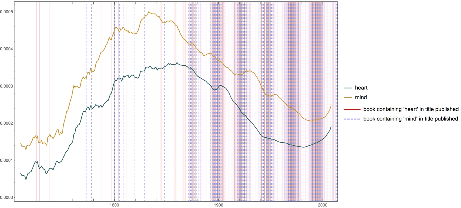
It is interesting to see that while the usage of both words decreased within the past century, books with titles containing both words have consistently been published with the century.
In other languages
Let's find out the heart-to-mind ratios and make plots for a few other languages. I have included English for comparison.
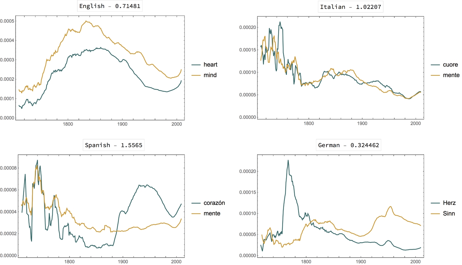
We see an even stronger correlation in Italian. I wonder if certain events led to the peak and decline of the use the words in the different languages. Most notably, in Spanish, Italian and German, could there have been a common cause for the rise and fall preceding the year 1800? I find the plot for the Spanish language the most interesting. Look closely at 1730 - 1760.
In famous texts
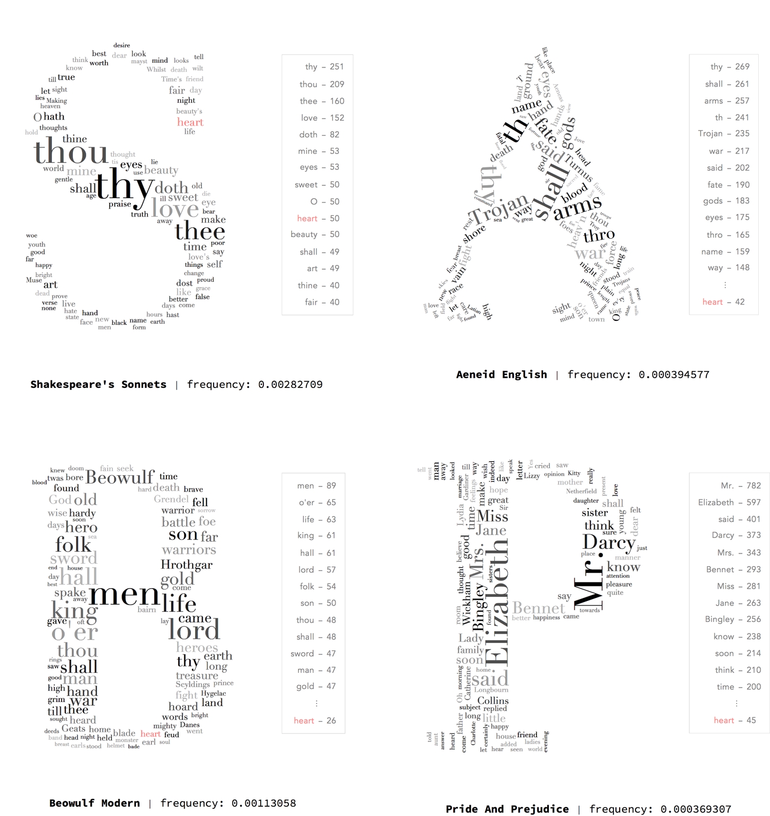
Using the tally of words in famous texts to generate a word cloud, in which the size and colour of a word are proportional to its frequency.
6. Anatomy
AnatomyData gives one access to a wealth of knowledge on the anatomy of the human body. Ways to access these information include using the various functions associated with real-world entities (Entity["AnatomicalStructure", "Heart"]) or the Interpreter function (e.g., Interpreter["AnatomicalStructure"]["heart"]).
By evaluating EntityList["AnatomicalStructure"] we see that there are up to 83,294 (as of 4 Nov. 2016) entities of the human anatomy to explore. I believe one can learn a lot about themselves by exploring just a few of these--in this post, we shall focus on the heart.
The human heart, like all other anatomical structures, is represented by an entity. This entity belongs to an entity class of organs. There are up to 112 different properties that can be explored for each organ. Some of these properties do not apply to certain organs. For example, the heart does not have any articulating bones within it or joints adjacent to it.
1(* entity of the human heart and a shallow view of its numerous features *)2Shallow[EntityClass["AnatomicalStructure", "Organs"]["Properties"]]

Property exploration
As we saw at the beginning of this section, there are numerous factual things one can find out about the heart right from the WL. Extracting properties from entities can be done using three distinct syntaxes: entity["PropertyDesired"], EntityValue[entity, "PropertyDesired"] and EntityProperty["entityTypeName", "PropertyDesired"][entity].
Yet another way to access information on anatomical structures in the human body is via the AnatomyData function (AnatomyData["entityName", "PropertyDesired"]). To demonstrate how these varying functions and syntaxes can be implemented, let's take a look at the length of the heart.
1s1 = heart["Length"];2s2 = EntityValue[heart, "Length"];3s3 = EntityProperty["AnatomicalStructure", "Length"][heart];4s4 = AnatomyData["Heart", "Length"];56(* results of syntaxes are the same *)7{SameQ[s1, s2, s3, s4], {s1, s2, s3, s4}}
{True, {12. cm, 12. cm, 12. cm, 12. cm}}
Property annotations
We've confirmed that the different methods lead to the same result. However, we do not know anything else about this figure, e.g., its source. Well, details about a property such as the source of information, definition and units (where applicable) can be obtained by using property annotations.
1(* function for displaying annotations of properties *)2showPropertyAnnotations[properties_List] := Block[{vals, otherProps},3 vals = "Values" -> ((# -> Block[{v = heart@#}, If[ListQ@v, Multicolumn[v, 3], v]]) & /@ properties);4 otherProps = Table[i -> ((# -> AnatomyData["Heart", #, i]) & /@ properties) /. {} | Missing[_] -> "-",5 {i, {"Qualifiers", "QualifierValues", "Description", "Definition", "Source", "Date", "PhysicalQuantity", "Unit"}}];6 Dataset@Association@MapAt[Association[#] &, Prepend[otherProps, vals], {;; , 2}]7 ];
Quantitative properties:
showPropertyAnnotations[{"Length", "Mass"}]

Qualitative properties:
showPropertyAnnotations[{"Shape", "Function"}]

Geometric properties
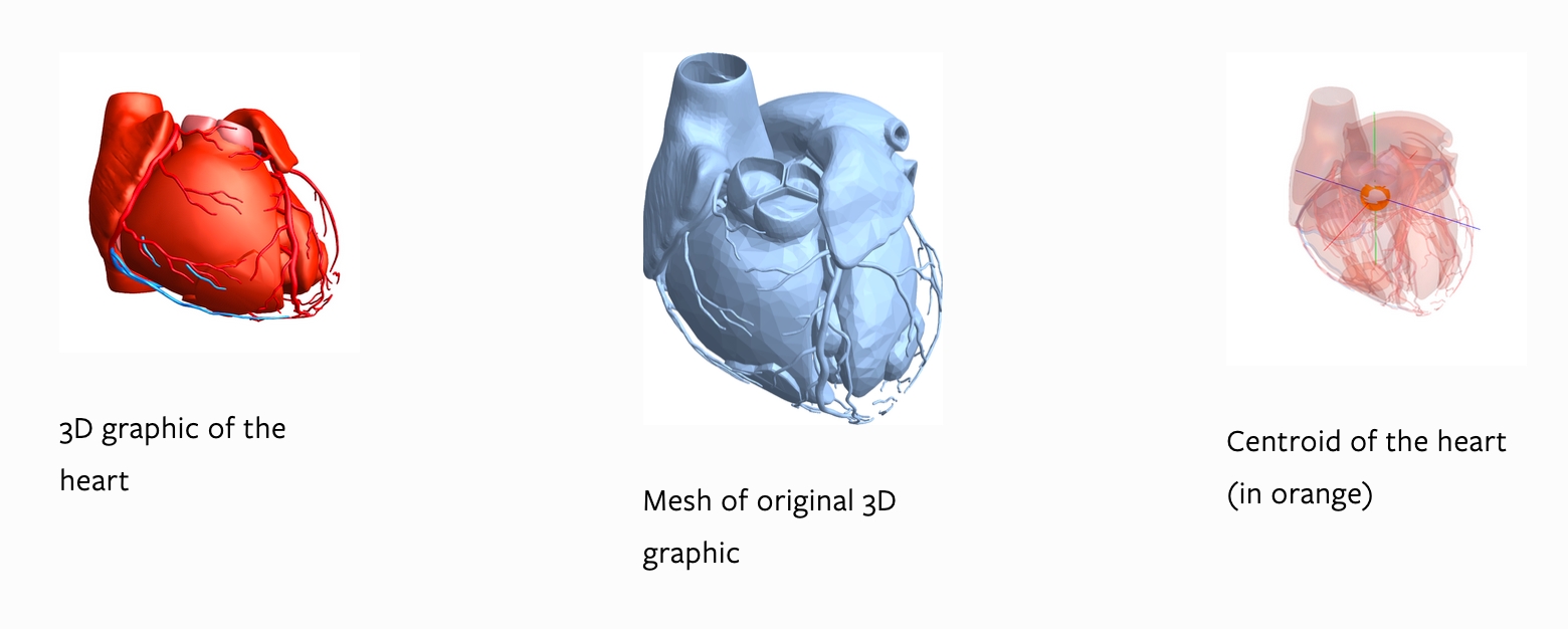
We can obtain a 3D model of the heart and its parts. Note that the 3D graphics generated in this subsection are heavily memory-intensive. The "MeshRegion" property gives a meshed region of the heart. Another way to do this is to use the DiscretizeGraphics function (i.e., DiscretizeGraphics[heart3D]) which can discretise a 2D or 3D graphic into a mesh region.
Pre-calculated properties relating to the mesh region, such as its area and centroid are also available. The centroid can also be found using the RegionCentroid function.
{heart["MeshArea"], cen = heart["RegionCentroid"]}
{113157. mm^2, {16.5384, -123.315, 1226.22}}
Nested property interactions
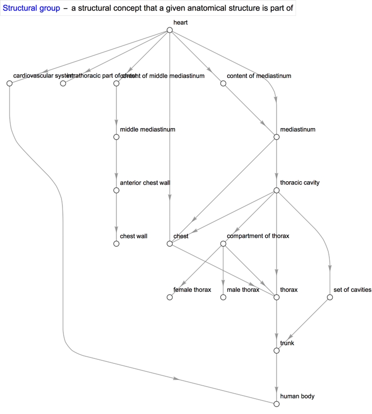
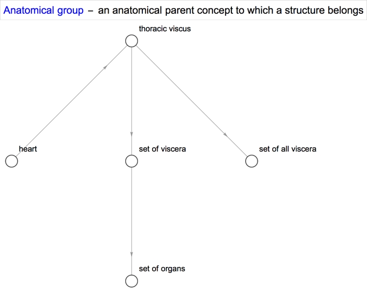
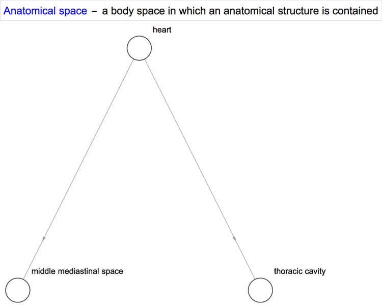
With some properties such as quantitative ones, we obtain a single value or an interval between two values. However, with others, we obtain a list of values. Sometimes, that property can be further applied to the items in the list. For example, the property "SystemicGroup" reminds us that the heart is a part of the cardiovascular system, which is itself a part of the human body.
We can represent this relationship in graphical form using NestGraph, which automatically forms connections between structures and the results returned when a certain property of theirs is queried. One of the amazing things about the Wolfram Language is the magnitude of its built-in functions and the diversity of its capabilities. They allow one to better focus one's efforts towards solving a problem and minimise the intermediate steps it takes to reach the solution.

Diseases/conditions of the heart
The richness of the information available for anatomical structures can be appreciated when one takes a look at the properties "Associated ICD-9" and "Associated ICD-10"—codes that characterise diseases. ICD-9 and ICD-10 stand for International Classification of Diseases Ninth and Tenth revision, respectively. According to the WHO, the first edition was originally designated 'the International List of Causes of Death' by the International Statistical Institute in 1893 [1]. Since its inception in 1948, the WHO has been responsible for revising and publishing the ICD, registering breakthroughs made in health and medical science over time [1].
ICD is the foundation for the identification of health trends and statistics globally, and the international standard for reporting diseases and health conditions. It is the diagnostic classification standard for all clinical and research purposes. ICD defines the universe of diseases, disorders, injuries and other related health conditions, listed in a comprehensive, hierarchical fashion...
— WHO
ICD-10 was put forward back in 1990 and ICD-11 is expected to be released in 2018 [1, 2]. For now, though, you can learn about the differences between ICD-9 and ICD-10 here. Note that the ICD codes we're dealing with here are associated only with the heart, and not other parts of the body. This table briefly compares the ICD-9 and -10.
1(* codes associated with the heart *)2Association[CommonName@# -> heart[#] & /@ {EntityProperty["AnatomicalStructure", "AssociatedICDNine"], EntityProperty["AnatomicalStructure", "AssociatedICDTen"]}

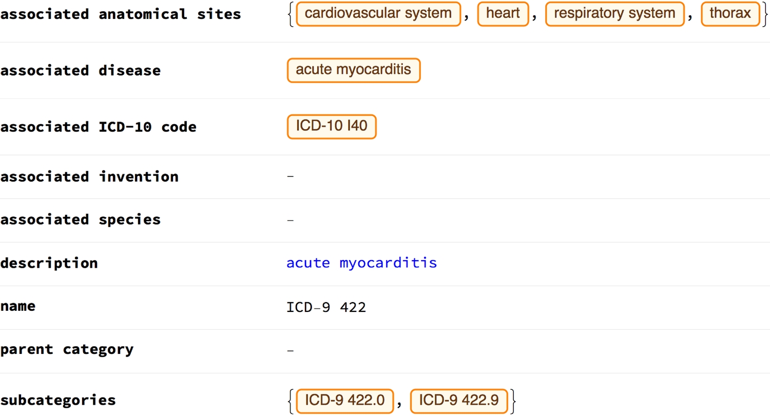
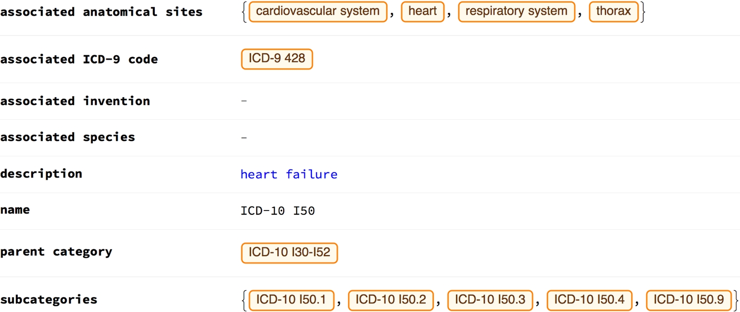
Example ICD codes and their properties:
Interactions between parts
In the previous section, we saw that some properties can be sought in a nested way. Delving further into such a property, this section will uncover the intricate interactions between anatomical structures of the hearts. The property in question is the constitutional parts of the heart.

We see that from the very first level, the heart constitutes 25 different parts. Now, we'll nestedly find out what each part is made up of. By iteration, I found that the deepest level of nesting possible for this particular organ, until one notices no changes, is seven! Manually finding these parts and creating edges between them to form a graph would be a tad difficult. Thankfully, the NestGraph function is perfectly apt for such a task. Just as they are linked directly to the heart, all constitutional parts of the heart will also be linked to their constituents, and so on.

There are 591 vertices (distinct constituent parts) in the graph! The depth of the nesting in various corners of the graph is reflected by its layout (asymmetric elongation). We can highlight the nest levels by colouring and resizing each vertex, according to its graph distance from the heart vertex. Also, we can show the distinction between parts that contain 'left' (hexagon) or 'right' (square), or neither (circle), by reshaping the vertices. The orange dotted lines show links between the heart and its immediate constitutional parts.
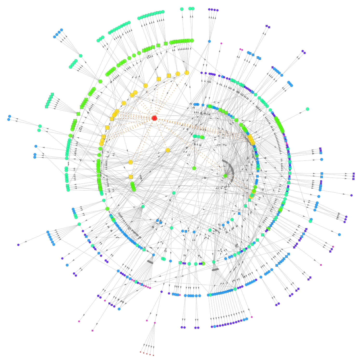
Back in section 3, we found the graph partition of a clustering tree. I attempted doing something similar here—finding the graph communities of parts within our styled graph. The result is very interesting. I cannot show the name of every vertex as the image will become beclouded. Some communities contain parts that mostly are of the same kind of structure, e.g. artery, cell/myocyte, septum, etc. Another thing to spot is the identical shape of vertices in some communities.

Common names
The common names of most parts contain the word 'of,' e.g. cytosol of the cardiac myocyte. Whereas some don't, other parts contain up to three 'of's in their names. This subsection analyses part names and how they relate to each other. I suspected that the names with the most number of 'of's will be the longest, or would at least have the most words in them.

We see that the longest name with up to three of's does have more words (13) than any other name. However, the longest name in the group of names with two of's has the longest name (88, by string length).
Where the name contains the word 'of,' the pieces linked by 'of' are hierarchical with respect to scale or some other property. For example, we can represent "fibrocollagenous connective tissue of myocardium of papillary muscle of right ventricle" simply with "x tissue of y muscle of z ventricle." If we replace the of's with undirected edges (where applicable) for all names, we'll obtain a large set of edges with which we can produce a visually rich graph of the connections between these hierarchies. Therefore, "x tissue of y muscle of z ventricle," for example, will be transformed into the edges {x tissue ●--> y muscle, y muscle ●--> z ventricle}.
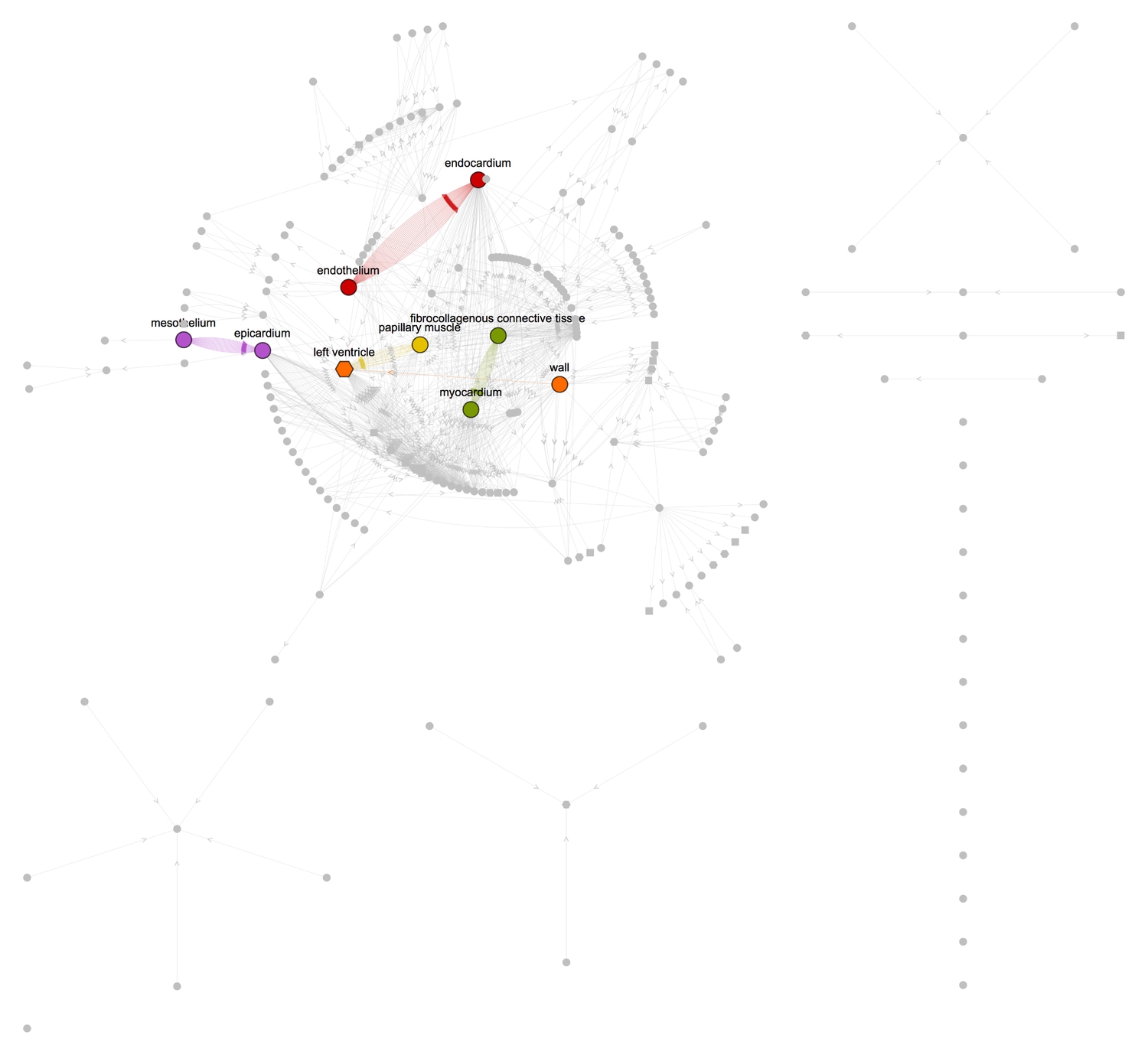
The graphs give a more lucid and articulate representation of how the constituents of the heart, large and minute, are interrelated. We can see for instance, from the graph, some pairs of vertices have many connections between them while some have just one. Taking a tally of all edges in the graph shows the most recurrently connected pairs of vertices. I have highlighted these vertices in the second graph above.
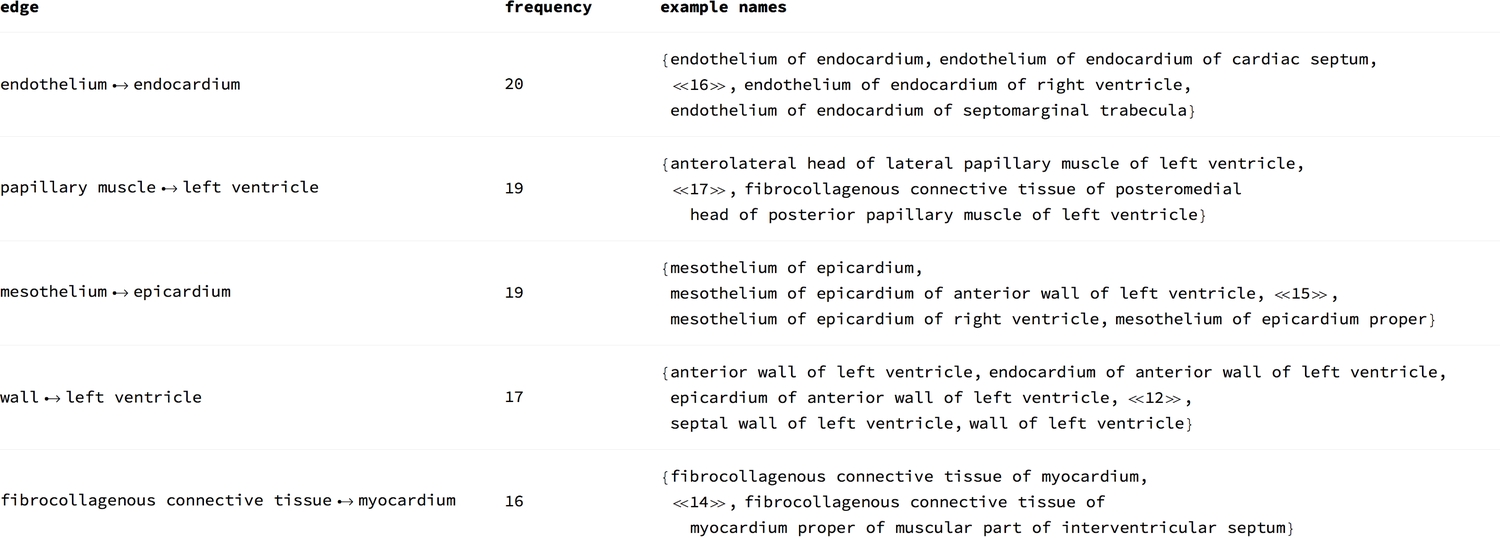
It is a wonder how vital a role these structures play, individually or together, for them to be this highly connected.
Graph measures
Distance matrix
We can find the graph distance matrix of the connections between all parts of the heart. This means finding the graph distance between each vertex and all other vertices—assigning a value of infinity where no path exists. The result is an intricate map of the heart that shows it from a different perspective.
The line across the main diagonal shows that all 591 vertices are connected to themselves, and thus have a distance of 0 between them. The horizontal line shows the heart's connection to all of its parts. There is no corresponding vertical line because the graph is a directed graph. The empty red spaces show a graph distance of infinity (i.e., no path found).
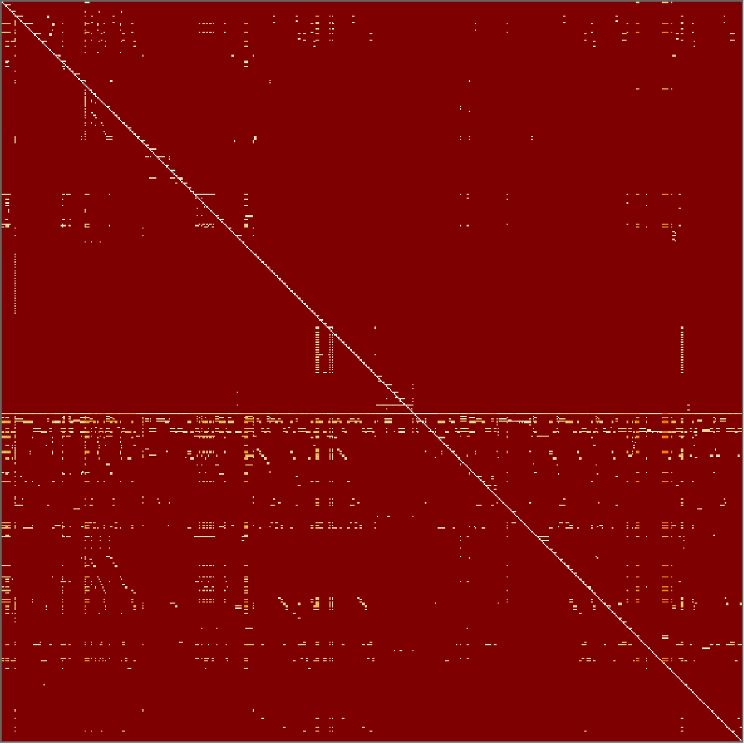
This visualisation shows some interesting patterns in the connections within the heart. Note that altering the sequence of the parts (e.g. sorting them alphabetically) will produce a different matrix, and thus, different patterns.
Degree centrality
The degree centrality of a vertex is the number of edges that lead to (In) or away from (Out) a the vertex. This measure is important in that it gives an idea of the sensitivity of vertices to the flow of something, either positive or negative within a network. However, the human heart is an organ made up of densely connected compact (and not separate) parts. Therefore, should something bad occur at a specific vertex, the spread is likely to be more erratic than the centrality measure's prediction.
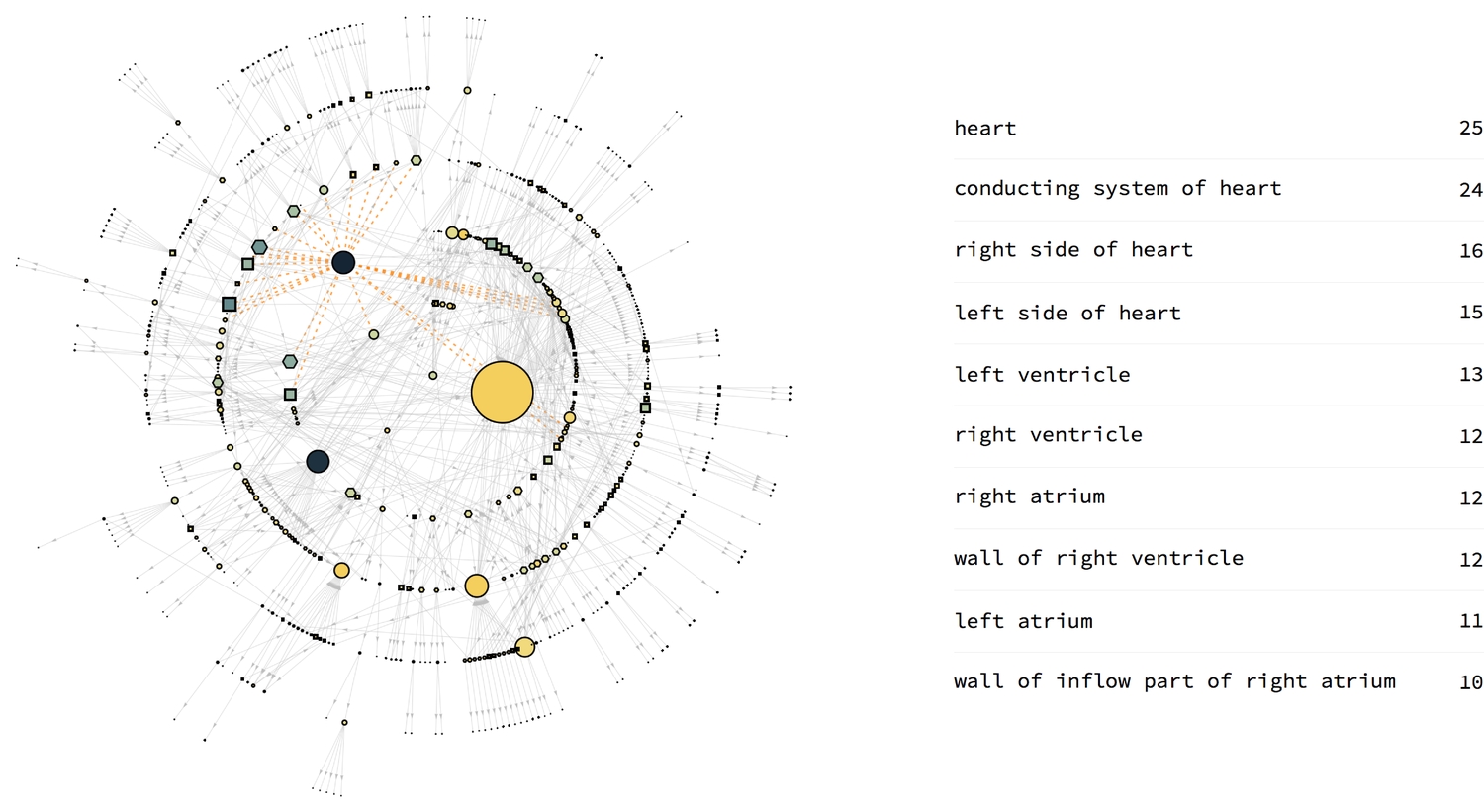
Closeness centrality
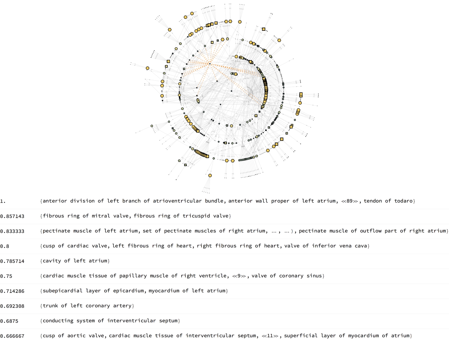
This is the average of the shortest possible distances between a vertex and every other vertex in the graph. It ranges between a minimum of 0 and a maximum of 1. A high closeness centrality value implies that the vertex can reach every other vertex more easily. For instance, if there are cancerous cells in a particular part of an organ, its centrality will determine how quickly the cells will spread out to other parts of the organ. Of course, in anatomy, a lot of other factors such as the size of the part, blood flow to and fro will influence the spread.
Betweenness centrality
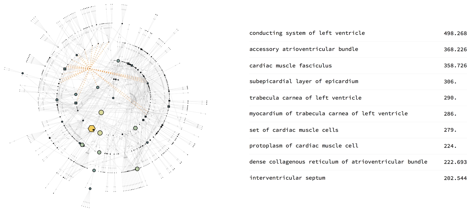
The betweenness centrality is a measure of the number of times a vertex lies on the shortest paths between other vertex pairs. Here, it shows the importance of vertices in carrying signals or nutrients around the heart. Cells lead to other smaller cellular components, and sets of cells lead to cells. Perhaps that explains why they've got high centralities. But there seems to be something peculiar about the left ventricle, which I am still trying to figure out. If the conducting system of the left ventricle lies on more shortest paths of vertex pairs than any other structure, then I suppose it is indeed conducting the workings of the heart.
Conclusion
The human heart is a beautifully complex organ. While the brain is associated with thinking, the heart is regarded by most as the source of feelings and emotions. Others think the two collectively form our emotions. This article has discussed my computational exploration of the human heart—beginning with semantics and ending with anatomy.
I have relied heavily on the knowledge-based Wolfram programming language, as both a source of data and a tool for data analysis. Although the sources of information aren't always included in the WL documentation, one can find most of them on Wolfram Alphait now allows you to compute things yourself, in the Wolfram Cloud. In fact, all of the code I have shown here can be evaluated directly from your browser. I shall soon upload computable notebooks for all EDAs so you can compute further as you read on.
As connected health advances, perhaps we will someday monitor or even visualise specific parts of intricate structures in our bodies such as the heart. I find the discourse on emotions in AI and robots very interesting. Given we aim to create these bits of intelligence and machines not only to match, amongst other things, our problem-solving aptitudes but to exceed them, will they someday share the feelings we have?
Writing this article and learning more about the "heart" was thoroughly enjoyable. I hope you have learned a thing or two from it and now see the heart in a different way than you used to. Keep exploring!
— MS