EDA I: The McClay Library

The McClay Library at Queen's University is an award-winning library. It contains more than a million volumes and more than 2,000 reader spaces. As the exam period approaches the number of occupants gradually rise. At its peak during exams, finding a PC or a seat can be quite difficult. The library provides occupancy data, showing the different floors, the number of available PCs on each, and the total number of occupants in the library. This service is updated once every 10 seconds and can be a useful guide when finding a place to study on a very busy day. I suppose that the information on the website is sourced from the library's controlled entry system.

Having been a student at Queen's for quite some time now, I am well aware of how the library can become saturated with rather disconcerted-looking students when occupancy peaks. I was curious to know how useful the occupancy information could be at such times. So I began exploring the website and later found a way to collect the data on it.

Throughout the summer exams period, I aim to gather as many data points as possible and play with the dataset. I hope to find something which can be beneficial to every Queen's student, in or out of exam season. In this post I shall discuss what I have done so far with the ever-growing dataset, and how I'm using the Wolfram Language and other technologies such as Wolfram Data Drop and Wolfram|Alpha to store and analyse it. I hope you find this both interesting and useful.

1. Simple display

I will begin by discussing how I accessed the occupancy information and visualised it the way I wanted. Two URLs are of interest here: http://go.qub.ac.uk/mcclay-availablepcs and http://go.qub.ac.uk/mcclay-occupancy. The former shows the number of available PCs on all floors while the latter shows the total number of people in the building.

1.1 Create dispay

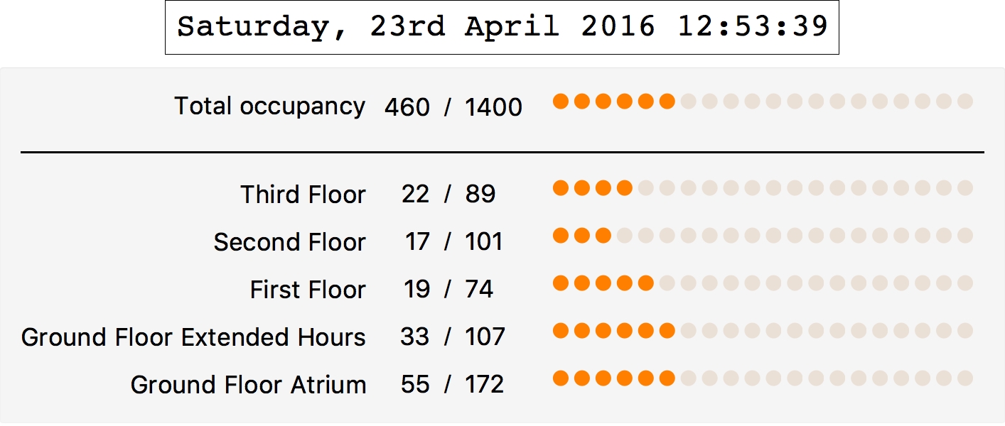
Combining data from both sources, we can create a simple interface similar to the one on the occupancy site. We'll first extract the data from our two sources and process it, and then represent occupancy and PC usage in the form of a horizontal gauge.

1display = Block[{
2  url = "https://www.qub.ac.uk/directorates/InformationServices/pcs/impero/",
3  url2 = "https://www.qub.ac.uk/directorates/InformationServices/pcs/sentry",
4  rawDataPCs, dataPCs, dataOccupancy, timeAndDate, mcclayLib,
5  currentOccupancy, maxOccupancy, gaugesPCs, gaugesOccupancy},
6
7 (* import info. from sites *)
8 rawDataPCs = Import[url];
9 (* extract useful info. *)
10 dataPCs = ImportString[rawDataPCs, "RawJSON"];
11 dataOccupancy = Import[url2];
12 {currentOccupancy, maxOccupancy} =
13  First /@ (
14    StringCases[
15       dataOccupancy, ___ ~~ "<" <> # <> ">" ~~ occ___ ~~
16         "</" <> # <> ">" ~~ ___ -> occ] & /@ {"occupancy",
17      "maxoccupancy"});
18 Row[{"Occupancy  ", Row[{currentOccupancy, maxOccupancy}, "/"]}];
19
20 (* extract time and date *)
21 timeAndDate = dataPCs["dateTimeNow"];
22 (* associate each floor with its info and sort list *)
23 mcclayLib =
24  With[{order = {"Ground Floor Atrium", "Ground Floor Extended Hours",
25       "First Floor", "Second Floor", "Third Floor"}},
26   {#[[1]], Row[{#[[3]] - #[[2]], #[[3]]}, " / "]} & /@
27    SortBy[Values[dataPCs["rooms"][[1 ;;, 2 ;; 4]]],
28     Position[order, #[[1]]] &]];
29
30 (* template for horizontal gauges *)
31 makeGauge[value_] :=
32  HorizontalGauge[value, {0, 1},
33   GaugeMarkers -> Placed[Graphics[Disk[]], "DivisionInterval"],
34   GaugeFrameSize -> None, GaugeFrameStyle -> None,
35   GaugeStyle -> {Orange, Lighter[Brown, .8]},
36   GaugeFaceStyle -> None,
37   ScaleRangeStyle -> {Lighter[Brown, #] & /@ {.9, .5}},
38   GaugeLabels -> {None, None},
39   TicksStyle -> None,
40   ScaleDivisions -> None, ScaleRanges -> None, ScalePadding -> 0
41   ];
42
43 (* gauges for PC usage on each floor *)
44 gaugesPCs = Table[
45   makeGauge[
46    N[(mcclayLib[[fl, 2, 1, 1]]/mcclayLib[[fl, 2, 1, 2]]), 2]],
47   {fl, Range@Length@mcclayLib}];
48
49 (* gauge for total number of occupants *)
50 gaugesOccupancy =
51  makeGauge[(FromDigits@currentOccupancy/FromDigits@maxOccupancy)];
52
53 (* put everything together *)
54 Column[{
55   Framed[timeAndDate,FrameStyle -> Directive[Black, Thin]],
56   Panel@Grid[
57     Prepend[
58      Reverse[Flatten /@
59        Transpose[{mcclayLib, gaugesPCs}]], {"Total occupancy",
60       Row[{currentOccupancy, maxOccupancy}, " / "], gaugesOccupancy}],
61     Alignment -> {"/", Center}, Dividers -> {None, {False, True}},
62     Spacings -> {Automatic, 2 -> 2}]
63   }, Alignment -> Center]
64 ]

Note that the values of all gauges are normalised between 0 and 1. This is what we get:

Occupancy and PC usage on all floors.

1.2 Deploy display to cloud

We can go ahead and deploy this to the Wolfram Cloud to make it accessible to every student.

1CloudDeploy[Delayed[
2  ExportForm[display,
3   "PNG", ImageFormattingWidth -> 400, ImageResolution -> 250],
4  UpdateInterval -> 20
5  ], "McClayLibraryOccupancy", Permissions -> "Public"]

The display then gets deployed to this website which automatically refreshes every 20 seconds:

https://www.wolframcloud.com/objects/user-8fa71eda-c6a8-4555-a394-46fd67a27d48/McClayLibraryOccupancy

and available here, also:

http://go.qub.ac.uk/mcclay-usagedisplay.

And of course, you can scan this QR code to get the info.

2. Collecting data

2.1 Create databin

To analyse the occupancy and PC usage over a while, we'll have to store the data somewhere. I chose to use the Wolfram Data Drop to do this. It allows you to easily create a databin and periodically add data to it using a custom API, email, Arduino, Raspberry Pi, IFTTT and even Twitter!

I used the Wolfram Langauge to create a databin, but you can also do this online:

1(* connect to Wolfram Cloud *)
2If[$CloudConnected == False, CloudConnect["username","password"],
3  Print["Connected to Wolfram Cloud."]];

1(* create bin *)
2libraryBin =
3 CreateDatabin[<|
4   "Name" -> "McClay Library",
5   "Interpretation" ->
6    {
7     "datetime" -> "DateTime",
8     "totalNum" -> Restricted["StructuredQuantity", "People"],
9     "grndFloorATR" -> Restricted["StructuredQuantity", "People"],
10     "grndFloorEXT" -> Restricted["StructuredQuantity", "People"],
11     "floor1" -> Restricted["StructuredQuantity", "People"],
12     "floor2" -> Restricted["StructuredQuantity", "People"],
13     "floor3" -> Restricted["StructuredQuantity", "People"],
14     "totalUsingPCs" -> Restricted["StructuredQuantity", "People"],
15     "totalNotUsingPCs" -> Restricted["StructuredQuantity", "People"]
16     },
17   "Administrator" -> $WolframID,
18   Permissions -> "Public"|>]

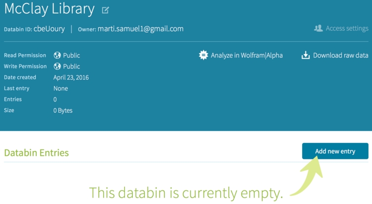
The databin is available to the "Public" and it automatically interprets and associates input values with their appropriate quantities, e.g., the number of "People" on each floor. Note that this databin is only temporary and expires a month from now. Data can not be added to it after it expires.

The following table explains what the inputs are:

datetime	date and time
totalNum	current library occupancy
grndFloorATR	Ground Floor Atrium
grndFloorEXT	Ground Floor (Extended Hours)
floor1	First Floor
floor2	Second Floor
floor3	Third Floor
totalUsingPCs	total no. of students using PCs
totalNotUsingPCs	total no. of students NOT using PCs

2.2 Properties of databin and metadata

To see properties of databin: Grid[Options[libraryBin] /. (property___ -> value___) -> {property, value},Frame -> All]

You can see the metadata of databin too: Column@Normal@libraryBin["Information"]

2.3 Prepare data for upload

Using the Wolfram Language, data is usually added to the bin in the form of an Association. Since we already know what the required inputs for our databin are, we can extract the occupancy and immediately process it into our desired association.

1getLibraryData[] := Block[
2   {
3 urlPCs =
4  "https://www.qub.ac.uk//directorates/InformationServices/pcs/impero/",urlOccupancy =
5  "https://www.qub.ac.uk//directorates/InformationServices/pcs/sentry",
6 rawDataPCs, PCsUsageData,OccupancyData, occ,
7 datetime, f0atr, f0ext, f1, f2, f3, totalUsingPCs, totalNotUsingPCs
8 },
9
10   rawDataPCs = Import[urlPCs];
11   PCsUsageData = ImportString[rawDataPCs, "RawJSON"];
12   datetime = PCsUsageData["dateTimeNow"];
13
14   (* occupancy *)
15OccupancyData = Import[urlOccupancy];
16occ = First@StringCases[OccupancyData, ___ ~~ "<occupancy>" ~~ occ___ ~~"</occupancy>" ~~ ___ :> FromDigits@occ];
17
18   (* PC usage on all floors *)
19{f0atr, f0ext, f1, f2, f3} =
20  Abs@With[{order = {"Ground Floor Atrium",
21       "Ground Floor Extended Hours", "First Floor", "Second Floor",
22       "Third Floor"}},
23    (#[[3]] - #[[2]]) & /@
24     SortBy[Values[PCsUsageData["rooms"][[1 ;;, {2, 3, 4}]]],
25      Position[order, #[[1]]] &]];
26totalUsingPCs = f0atr + f0ext + f1 + f2 + f3;
27totalNotUsingPCs = occ - totalUsingPCs;
28
29   (* our desired association *)
30<|"datetime" -> datetime, "totalNum" -> occ, "grndFloorATR" -> f0atr,
31 "grndFloorEXT" -> f0ext, "floor1" -> f1, "floor2" -> f2,
32 "floor3" -> f3, "totalUsingPCs" -> totalUsingPCs,
33 "totalNotUsingPCs" -> totalNotUsingPCs|>
34  ];

This version handles failure which arises from lack of internet connection, etc.

1getLibraryData2[] := Block[
2   {
3    urlPCs = "https://www.qub.ac.uk//directorates/InformationServices/pcs/impero/",
4    urlOccupancy = "https://www.qub.ac.uk//directorates/InformationServices/pcs/sentry",
5    rawDataPCs, PCsUsageData, PCsUsageDataAssoc,
6    OccupancyData, occ,
7    datetime, f0atr, f0ext, f1, f2, f3, totalUsingPCs, totalNotUsingPCs
8    },
9
10   (* import all data *)
11   rawDataPCs = Check[Import[urlPCs], $Failed];
12   OccupancyData = Check[Import[urlOccupancy], $Failed];
13
14   (* import failure criteria *)
15   ImportFailedQ[dataToImport_] := FailureQ[dataToImport];
16
17   (* proceed (if data is imported successfully; all are free from failure) *)
18   If[FreeQ[{ImportFailedQ@rawDataPCs, ImportFailedQ@OccupancyData},
19     True],
20    (
21     (* extract PC usage, timestamp & occupancy data *)
22
23     PCsUsageData = ImportString[rawDataPCs, "RawJSON"];
24     datetime = PCsUsageData["dateTimeNow"];
25     occ =
26      First@ StringCases[
27        OccupancyData, ___ ~~ "<occupancy>" ~~ occupancy___ ~~
28          "</occupancy>" ~~ ___ :>
29         If[occupancy == "NA", Missing["NotAvailable"],
30          FromDigits@occupancy]];
31
32     (* processing *)
33     PCsUsageDataAssoc =
34      Cases[PCsUsageData[["rooms"]][[;; , 2 ;; 4]],
35        KeyValuePattern[{"roomDescription" -> x__,
36           "freeCount" -> y_ /; y >= 0,
37           "totalCount" -> z_ /; z >= 0}] :> (x -> (z - y))] //
38       Association;
39
40     {f0atr, f0ext, f1, f2, f3} =
41      With[{order = {"Ground Floor Atrium",
42          "Ground Floor Extended Hours", "First Floor",
43          "Second Floor", "Third Floor"}},
44       Lookup[PCsUsageDataAssoc, #, Missing["NotAvailable"]] & /@
45        order];
46
47     totalUsingPCs = With[{floors = {f0atr, f0ext, f1, f2, f3}},
48         If[FreeQ[floors, #], Total@floors, #]
49         ] &@Missing["NotAvailable"];
50     totalNotUsingPCs =
51      If[totalUsingPCs === #, #, occ - totalUsingPCs] &@
52       Missing["NotAvailable"];
53
54     (* our desired association *)
55     <|"datetime" -> datetime,
56      "totalNum" -> occ, "grndFloorATR" -> f0atr,
57      "grndFloorEXT" -> f0ext, "floor1" -> f1, "floor2" -> f2,
58      "floor3" -> f3, "totalUsingPCs" -> totalUsingPCs,
59      "totalNotUsingPCs" -> totalNotUsingPCs|>
60     )
61    (* else do nothing - upload skipped *)
62    ]
63   ];

Running this gets the data and creates an association we can directly send to our databin. For example, evaluating getLibraryData[] gives:

<|"datetime" -> "Saturday, 23rd April 2016 14:40:05", "totalNum" -> 630, "grndFloorATR" -> 88, "grndFloorEXT" -> 50, "floor1" -> 24, "floor2" -> 25, "floor3" -> 33, "totalUsingPCs" -> 220, "totalNotUsingPCs" -> 410|>

Uploading data

There are various ways to upload extracted data to our bin. We'll do this using the Wolfram Language since our data will first need to be extracted from a website.

3.1 Using a scheduled task

Scheduled tasks are great for running code in the background. QUB updates the data on the occupancy website once every 10 seconds. However, a basic Wolfram Data Drop only allows a maximum of 60 data entries per hour. So we'll upload our data once every minute to add as much as possible to the databin each hour. Note that the short ID for our databin is cbeUoury.

1libraryBin = Databin["cbeUoury"]
2RunScheduledTask[(
3  assoc = getLibraryData[];
4  DatabinAdd[libraryBin, assoc]), 60]

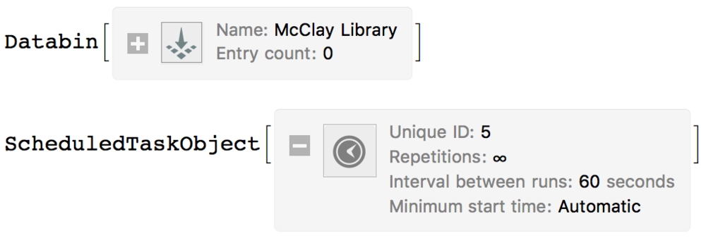
As long as we allow this to run without interrupting the task or closing Mathematica, it'll run forever. This is fantastic, given that every Raspberry Pi comes with Mathematica pre-installed! We can also add data to the bin using a custom API, Arduino and other different methods.

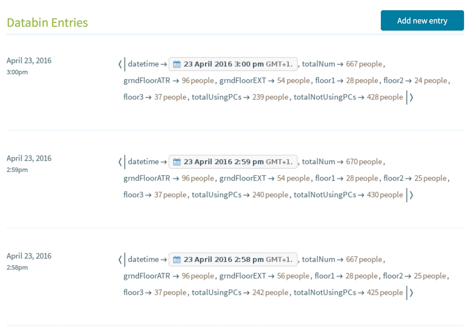
After a few minutes (and entries) our data can be viewed on the databin site. You can deploy your scheduled task to the Wolfram Cloud and it'll keep running until you choose to stop it. Although a paid subscription is required to use this service. This will be ideal for gathering data over a lengthy period, which is what I aim to do. I don't have a paid subscription at the moment but will look into getting one. For now, data uploads will be made from Mathematica on my PC or using a Raspberry Pi, or an Intel Edison.

After a few minutes (and uploads) we can view our data.

3.2 Cloud-based scheduled task

If we're deploying our scheduled task to run autonomously in the cloud, we'd run the following code:

1dataUploadCloudObject = Block[{shortid = "cbeUoury", databin, assoc},
2  databin = Databin[shortid];
3  CloudDeploy[ScheduledTask[
4  (assoc = getLibraryData[]; DatabinAdd[databin, assoc]),
5   600],"McClayLibraryDataUpload", Permissions -> "Private"
6   ]]

4. Data Analysis

I ran the program pretty much throughout the exam period with short intervals of inactivity. The entries amassed into a dataset large enough to spot trends and run some analyses.

4.1 Dataset

Let's see an overview of the data we have collected so far:

1(* Data collected so far *)
2libraryBin = Databin["cK8HWZj4"];
3dataEntriesThusFar := libraryBin["Entries"];

1(* Delete Null, Missing and Negative cases... Sometimes we get negative cases when the number of available PCs isn't updated correctly. *)
2dataEntriesThusFar =  DeleteCases[dataEntriesThusFar, Null | getLibraryData2[], {1}];
3dataEntriesThusFar = DeleteCases[dataEntriesThusFar, _Missing | _?Negative | getLibraryData2[], {2}]

List of all entries, thus far.

View the dataset.

dataset = Dataset[dataEntriesThusFar]

Dataset

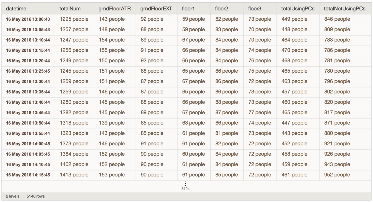
Now we have a continuously growing dataset — we can run some analysis and see if we find anything meaningful/useful out of it.

4.2 Basic Stats

Find the minimum, maximum, standard deviation, etc of each library location:

1Module[{funcs = {"Location", Mean, StandardDeviation, Median, Max,
2    Min}},
3 Prepend[Flatten@{#,
4       Table[dataset[
5         IntegerPart@func[Cases[#, _?QuantityQ]] &, #1], {func,
6         Rest@funcs}]} & /@ {"totalNum", "totalUsingPCs","totalNotUsingPCs", "grndFloorATR", "grndFloorEXT", "floor1", "floor2", "floor3"},
7   ToString /@ funcs] // Dataset
8 ]

Visualise the stats using box charts.

1makeBoxChart[labels_] := Block[{data},
2  data = Table[DeleteMissing@Normal@dataset[[All, i]], {i, labels}];
3  BoxWhiskerChart[data,
4   {{"Outliers", Large}, {"Whiskers", Thin}, {"Fences", Thin}},
5   AspectRatio -> 1/2, ChartLabels -> labels, ChartStyle -> "StarryNightColors", BarOrigin -> Left,
6   BarSpacing -> .5, PerformanceGoal -> "Quality", ImageSize -> 400]];
7
8   makeBoxChart[#] & /@ {{"totalNum", "totalUsingPCs",
9    "totalNotUsingPCs"}, {"grndFloorATR", "grndFloorEXT", "floor1", "floor2", "floor3"}} // gridOfTwoItems

Basic stats

Box charts

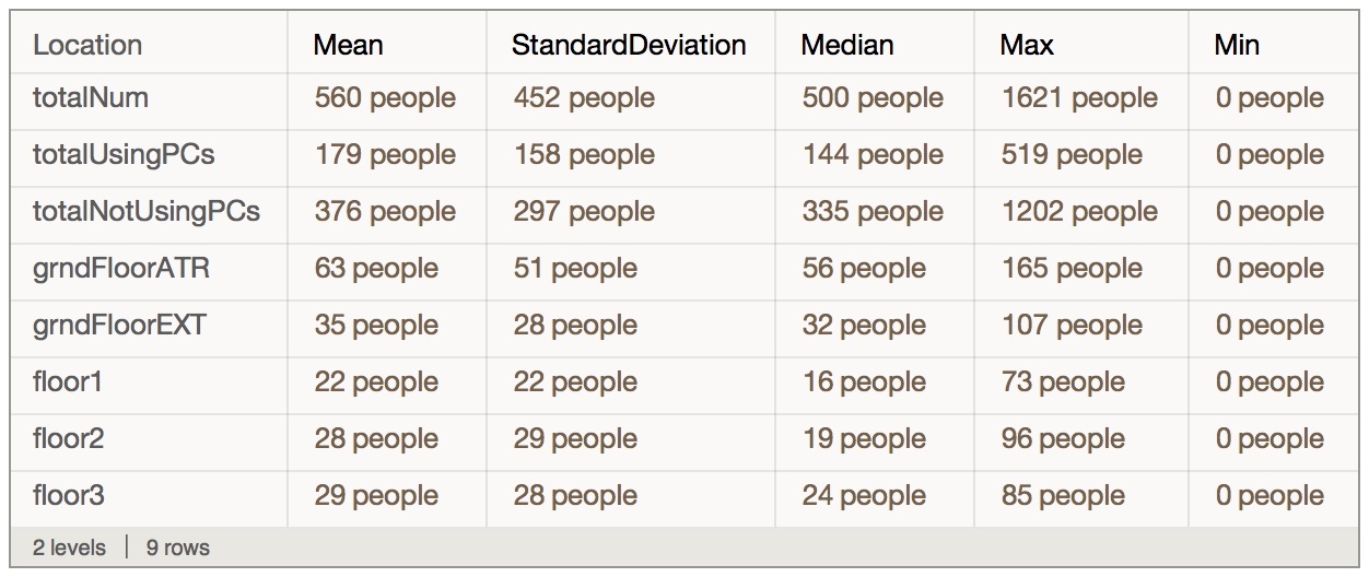
Visualise the mean number of people using PCSs on each floor.

1Table[(dataset[
2    BarChart[Floor@Mean[QuantityMagnitude[DeleteMissing[#, 1, Infinity]]],
3      BarOrigin -> Left, ChartStyle -> "StarryNightColors", ChartLegends -> Automatic, PlotLabel -> "Mean number of people\n", PlotTheme -> "Detailed"] &, i]),
4  {i, {{"grndFloorATR", "grndFloorEXT", "floor1", "floor2",
5     "floor3"}, {"totalUsingPCs", "totalNotUsingPCs"}}}] // gridOfTwoItems

Mean number of PCs in use and free on all levels.

To find when the library had the highest number of people in it:

Query[MaximalBy[#totalUsingPCs &]] @ dataset

On 17 May, at about 11.20 am was there was the highest number of occupants over the exam period.

4.3 Time series analysis

Extract the time series of library floors and remove the last time series from the list. This time series holds failed entries that were uploaded to the databin before I made getLibraryData2.

tseries = Delete[libraryBin["TimeSeries"], -1];

1makeDatePlot[series_List] :=
2  Block[{colourScheme = Take[ColorData[89, "ColorList"], Length[series]]},
3   DateListPlot[(QuantityMagnitude[tseries[#1]] &) /@ series,
4    AspectRatio -> 1/\[Pi], PlotStyle -> ({#1,
5         Directive[AbsoluteThickness[0.75`], Opacity[1]]} &) /@ colourScheme,
6    PlotLabels -> MapThread[Style, {(tseries[#1]["LastValue"] &) /@ series, colourScheme}], Filling -> Bottom,
7    PlotLegends -> Placed[SwatchLegend[colourScheme, series, LegendLayout -> "Row"], Bottom],
8    FrameLabel -> Automatic, Frame -> True,
9    FrameTicks -> {{Automatic, None}, {All, Automatic}},
10    GridLines -> Automatic, ImageSize -> 800,
11    PlotRangePadding -> {0, {0, Automatic}},
12    TargetUnits -> {"DimensionlessUnit", "People"}]];

1{makeDatePlot[{"floor3", "floor2", "floor1", "grndFloorEXT", "grndFloorATR"}],
2  makeDatePlot[{"totalNum", "totalUsingPCs", "totalNotUsingPCs"}]} // Column

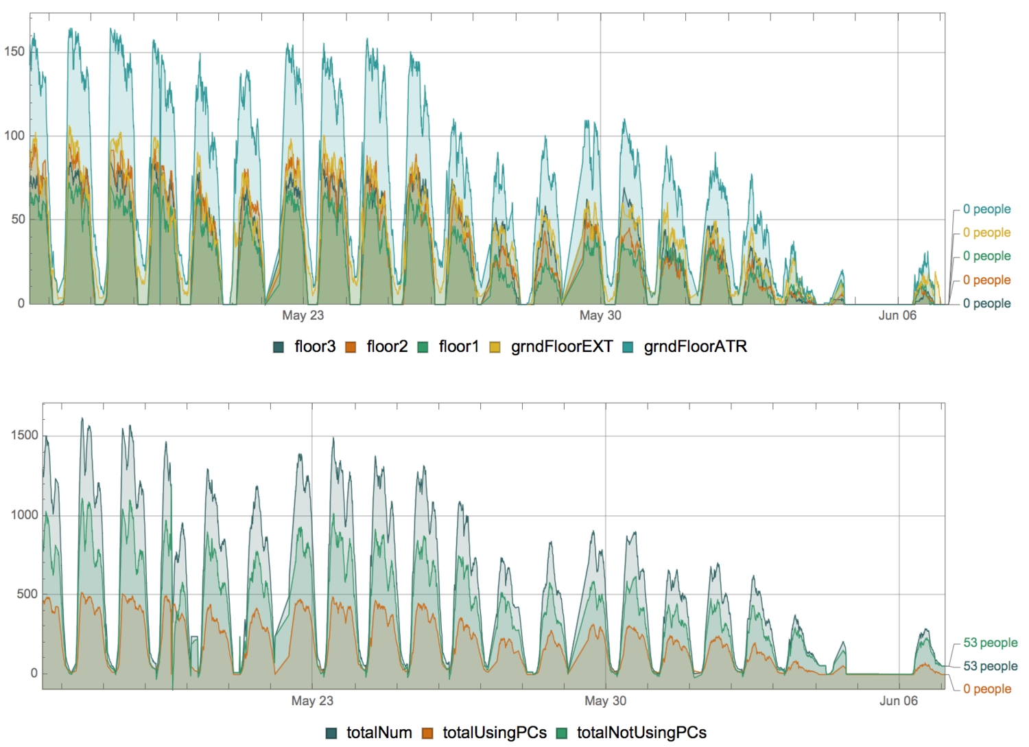
Library occupancy and PC usage trends. (Note that I stopped running the program for a while after exams, hence the flat gap. I ran it again to after some days to carry out some tests.)

Let's see the timespan of entries, and the latest entry to the databin with its metadata.

1Column@Normal@libraryBin["Latest"]
2Grid@Transpose[{{"First Entry", "Last Entry"}, libraryBin["TimeInterval"]}]

4.4 Location

See where entries were uploaded from.

1(* list of geo locations for all entries in the databin *)
2geoLocations = libraryBin["GeoLocations"];
3geoLocTallyAssoc = Tally[geoLocations] /. {g_GeoPosition, c_} :> {g -> c} // Flatten //Association;
4
5(* plot geo locations on a map *)
6pinToMap[highText_] := Column[{highText,
7    Graphics[
8     GraphicsGroup[{FaceForm[{Orange, Opacity[.8]}],
9       FilledCurve[{{Line[
10           Join[{{0, 0}}, ({Cos[#1], 3 + Sin[#1]} &) /@ Range[-((2 \[Pi])/20), \[Pi] + (2 \[Pi])/20, \[Pi]/20], {{0, 0}}]]},
11              {Line[(0.5 {Cos[#1], 6 + Sin[#1]} &) /@
12             Range[0, 2 \[Pi], \[Pi]/20]]}}]}], ImageSize -> 15]}, Alignment -> Center];
13
14findNearestCity[geoCoords_] :=
15  Row[{First[GeoNearest[Entity["City"], geoCoords]], " (",
16    geoLocTallyAssoc@geoCoords,
17    If[geoLocTallyAssoc@geoCoords == 1, " entry", " entries"], ")"}];
18
19GeoGraphics[(GeoMarker[#[[1, 1]], pinToMap[#], "Alignment" -> Bottom,
20         "Scale" -> Scaled[1]] &[findNearestCity@#1]) & /@ (First /@
21      Tally[geoLocations]) & /@ (First /@ Tally[geoLocations]),
22 GeoRange -> "World", GeoProjection -> "Equirectangular",
23 PlotRangePadding -> Scaled[.05], ImageSize -> 750]

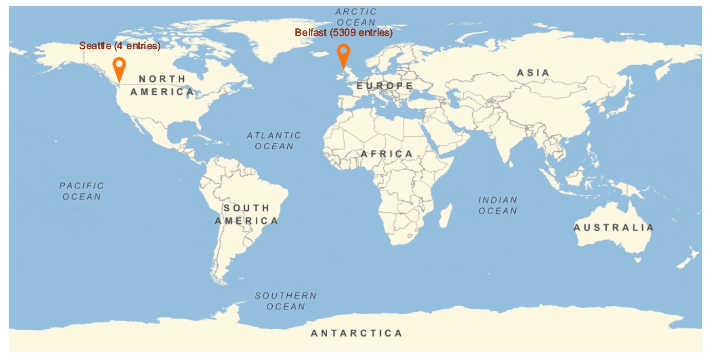
Most of the entries were from my PC (Belfast) while a few were uploaded by calling a custom API I created (I assume the server(s) that handled these are based in Seattle).

5. Distributions

In this section, I'll discuss my attempt in finding the daily distributions of people using the library and the PCs in it. I followed William Sehorn's methods in this article to find and visualise the distributions.

5.1 Date-value pairs

Shown below are the timestamps and values of entries.

1(* convert date-objects to date-strings *)
2dateValuePairs = (tseries["totalNum"]["DatePath"]) /. {x_,
3     y_} :> {DateString@x, QuantityMagnitude@y};
4RandomSample[dateValuePairs, 10]
5
6(* Reformat date-strings to date-lists *)
7dateValuePairs =
8 dateValuePairs /. {date_, value_} :> {DateList@date, value}
9
10(* total number of entries *)
11Length@dateValuePairs

We have 4866 date-value pairs in total.

5.2 Daily occupancy distributions

We’ll group all entries into 5-minute intervals over 24 hours:

timeIntervals = Tuples[{Range[0, 23], Range[0, 55, 5]}]; timeIntervals[[;; 12]]

Find the number of people within each time interval, over the entire data-gathering period:

1Clear[addOccupancyToTimeInterval, OccupancyAtTimeInterval];
2OccupancyAtTimeInterval[_] = 0;
3
4addOccupancyToTimeInterval[{__, hour_, minute_, _}, occupancyCount_] := OccupancyAtTimeInterval[{hour, minute}] += occupancyCount;
5
6addOccupancyToTimeInterval @@@ dateValuePairs;

For example, we can find the total number of people for 5-past-noon, over the entire period.

OccupancyAtTimeInterval[{12, 5}]

We can see that the total number of people between noon and 5-past-noon is 1575.

We can now plot the number of people over 5-minute intervals for the entire day.

1OccupancyDistributionData = OccupancyAtTimeInterval /@ timeIntervals;
2OccupancyDistributionData =
3  RotateLeft[OccupancyDistributionData, 12*6];

1barChartStyleOptions = With[{yticks =
2     Map[{#*12,
3        DateString[3600*(# + 6), {"Hour12Short", " ", "AMPM"}]} &,
4      Range[0, 24, 2]]},
5   {
6    AspectRatio -> 1/5, Frame -> True, FrameTicks -> {{None, None}, {yticks, None}},
7     FrameStyle -> GrayLevel[0.75], FrameTicksStyle -> Black,
8    GridLines -> {Range[24, 11*24, 24], None}, GridLinesStyle -> GrayLevel[0.87],
9    Ticks -> None,
10    BarSpacing -> 0,
11    PlotRange -> {{1, 288}, All},
12    PlotRangePadding -> {{1, 0}, {1, Scaled[.15]}},
13    ImagePadding -> {{12, 12}, {20, 0}}
14    ChartElementFunction ->
15     ChartElementDataFunction["SegmentScaleRectangle",
16      "Segments" -> 20, "ColorScheme" -> "DeepSeaColors"],
17    PerformanceGoal -> "Speed", ImageSize -> 750,
18    }
19   ];
20
21BarChart[OccupancyDistributionData, barChartStyleOptions]

Distribution of occupants over 24 hours.

So… Is it the same pattern every day? Apparently not.

1(* remove June entries *)
2totalNumTimeSeries =
3 TimeSeriesWindow[tseries["totalNum"], {{2016, 5, 16}, {2016, 5, 31}}];
4wd = WeightedData[totalNumTimeSeries["Dates"],
5   totalNumTimeSeries["Values"]];
6DateHistogram[wd, "Day", DateReduction -> "Week",
7 ColorFunction -> "StarryNightColors"]

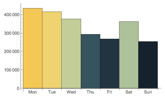
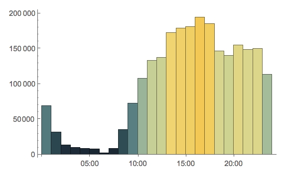
Oddly, there’s a deviation from the decreasing-in-number trend on Saturday.

If we reduce the histogram down to the span of a day, we get a clearer picture of the flow of people, in and out of the library:

DateHistogram[wd, “Hour”, DateReduction -> “Day”, ColorFunction -> “StarryNightColors”]

We see a smoother increase and fall here, as compared to the previous plot because the data is binned hourly here, and by minute in the previous one.

5.3 Array plot of occupants by time

1arrayData = dateValuePairs[[All, 2]];
2arrayData = Partition[arrayData, 12*24];
3arrayData = Transpose[Reverse /@ arrayData];
4
5arrayPlotStyleOptions = Module[{startDate, endDate, xticks, yticks},
6   startDate = dateValuePairs[[1, 1, ;; 3]];
7   endDate = dateValuePairs[[-1, 1, ;; 3]];
8   yticks = {#*12,
9       DateString[(24 - #)*3600, {"Hour12Short", " ", "AMPM"}]} & /@
10     Range[0, 24, 4];
11   xticks =
12    With[{month = Take[DatePlus[startDate, {#, "Month"}], 2]},
13       {QuantityMagnitude@DateDifference[startDate, month],
14        DateString[month, "MonthName"]}
15       ] & /@
16     Range[0, First@DateDifference[startDate, endDate, "Month"] + 1];
17   {
18    AspectRatio -> 1/4,
19    Frame -> True, FrameTicks -> {{yticks, None}, {xticks, None}},
20    FrameStyle -> GrayLevel[.75], FrameTicksStyle -> Black,
21    ImageSize -> 450, PlotRangePadding -> {{0, 0}, {0, 1}},
22    ColorFunction -> "StarryNightColors"
23    }
24   ];
25
26ArrayPlot[arrayData, arrayPlotStyleOptions]

Occupancy vs time

5.4 Daily and monthly distributions

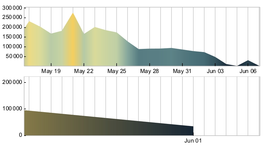
1(* Auxiliary functions *)
2occupancyDataEntryToDay[{{year_, month_, day_, __}, _}] := {year,
3   month, day};
4occupancyDataEntryToMonth[{{year_, month_, __}, _}] := {year, month};
5getDailyTotals[data_] :=
6 Module[{groupedByDay},
7  groupedByDay = GatherBy[data, occupancyDataEntryToDay];
8  Map[Total@#[[All, 2]] &, groupedByDay]
9  ]
10
11(* daily distribution *)
12dailyOccupancyTotals = getDailyTotals[dateValuePairs];
13days = DeleteDuplicates[occupancyDataEntryToDay /@ dateValuePairs];
14dailyPlotData = Transpose[{days, dailyOccupancyTotals}];
15
16(* plotting style options common to daily and monthly distribution plots *)
17sharedDateListPlotStyleOptions =
18  {
19   Joined -> True, Filling -> Axis, ImageSize -> 450, Frame -> True,
20   FrameStyle -> GrayLevel[.75], FrameTicksStyle -> Black,
21   FillingStyle -> Automatic, PlotStyle -> Directive[Thickness[.002], Black],
22   PlotRange -> {libraryBin["TimeInterval"], {0, All}},
23   GridLines -> {DayRange[First@#, Last@#] &@
24      libraryBin["TimeInterval"](*{2016,#,1}&/@Range[1,12]*), None},
25   GridLinesStyle -> GrayLevel[.8]
26   };
27
28(* plotting options for daily distribution *)
29dailyDateListPlotStyleOptions =
30  With[{padding = .1},
31   {
32    FrameTicks -> {{Rest@
33        FindDivisions[{0, (1 + padding)*Max@dailyOccupancyTotals, 1}, 8], None},
34       {DateString[#, {"DayShort", " ", "MonthNameShort"}] & /@
35          DateRange[First@#, Last@#, Quantity[3, "Days"]] &@
36        libraryBin["TimeInterval"][[;; , 1]], None}},
37    PlotRangePadding -> {{0, 0}, {0, Scaled[padding]}}, ImagePadding -> Automatic, AspectRatio -> 1/4, ColorFunction -> "StarryNightColors"
38    }
39   ];
40
41(* daily distribution plot *)
42dailyPlot = DateListPlot[dailyPlotData, sharedDateListPlotStyleOptions, dailyDateListPlotStyleOptions]

Daily distribution

For monthly distribution:

1groupedByMonth = GatherBy[dateValuePairs, occupancyDataEntryToMonth];
2monthlyOccupancyAverages =
3  Map[Mean@getDailyTotals@# &, groupedByMonth];
4months = DeleteDuplicates[occupancyDataEntryToMonth /@ dateValuePairs];
5monthlyPlotData = Transpose[{months, monthlyOccupancyAverages}];
6
7(* monthly distribution plotting options *)
8monthlyDateListPlotStyleOptions =
9  With[{padding = .3},
10   {
11    FrameTicks -> {{Most@
12        FindDivisions[{0, (1 + padding)*Max@monthlyOccupancyAverages,
13          1}, 4], None}, {months, None}},
14    PlotRangePadding -> {{0, 0}, {0, Scaled[padding]}},
15    ImagePadding -> Automatic, AspectRatio -> 1/4, ColorFunction -> "StarryNightColors"
16    }
17   ];
18
19monthlyPlot = DateListPlot[monthlyPlotData, sharedDateListPlotStyleOptions, monthlyDateListPlotStyleOptions]

Monthly distribution

Daily and monthly distributions stacked together:

Column[{dailyPlot, monthlyPlot}, Spacings -> 0]

5.5 Distributions for each floor

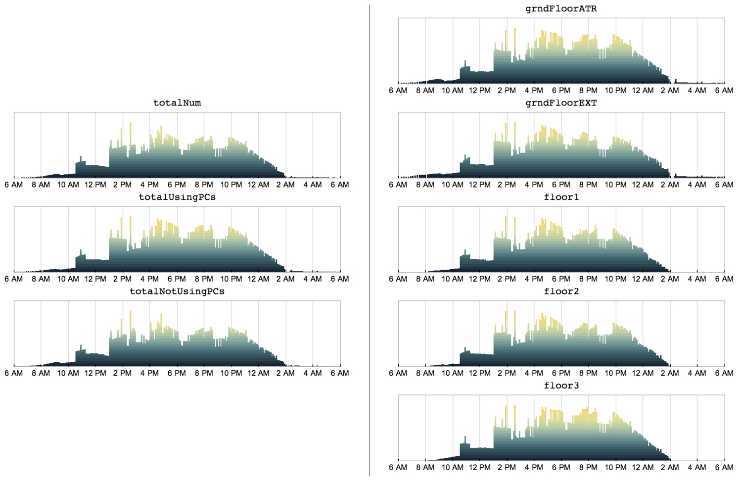
Lastly, we want to see how the PC usage evolves over a day on each floor. To generate the following plots, I combined pieces of code from previous sections and formed a function that could be used repeatedly.

1plotDailyDistribution[timesries_] := Block[
2  {dateValuePairs, timeIntervals, OccupancyAtTimeInterval,
3   addOccupancyToTimeInterval, OccupancyDistributionData,
4   barChartStyleOptions},
5
6  (* convert date-objects to date-strings *)
7
8  dateValuePairs = (tseries[timesries]["DatePath"]) /. {x_,
9      y_} :> {DateString@x, y};
10  (* Reformat date-strings to date-lists *)
11
12  dateValuePairs[[All, 1]] = DateList /@ dateValuePairs[[All, 1]];
13
14  (* create 5-minute intervals over 24 hours *)
15
16  timeIntervals = Tuples[{Range[0, 23], Range[0, 55, 5]}];
17
18  OccupancyAtTimeInterval[_] = 0;
19  addOccupancyToTimeInterval[{__, hour_, minute_, _}, stepCount_] :=
20
21     OccupancyAtTimeInterval[{hour, minute}] += stepCount;
22  addOccupancyToTimeInterval @@@ dateValuePairs;
23
24  OccupancyDistributionData = OccupancyAtTimeInterval /@ timeIntervals;
25  OccupancyDistributionData =
26   RotateLeft[OccupancyDistributionData, 12*6];
27  (* averaged daily distribution of occupancy *)
28
29  (* barchart styling options *)
30  barChartStyleOptions = With[{yticks =
31      Map[{#*12,
32         DateString[3600*(# + 6), {"Hour12Short", " ", "AMPM"}]} &,
33       Range[0, 24, 2]]},
34    {
35     AspectRatio -> 1/5, Frame -> True, FrameTicks -> {{None, None}, {yticks, None}}, FrameTicksStyle -> Black, GridLines -> {Range[24, 11*24, 24], None},
36     GridLinesStyle -> GrayLevel[0.87], PlotRange -> {{1, 288}, All}, Ticks -> None, BarSpacing -> 0,
37     PlotRangePadding -> {{1, 0}, {1, Scaled[.15]}}, ChartElementFunction ->
38      ChartElementDataFunction["SegmentScaleRectangle",
39       "Segments" -> 20, "ColorScheme" -> "StarryNightColors"], PerformanceGoal -> "Quality", ImageSize -> 450, FrameStyle -> GrayLevel[0.75], ImagePadding -> {{12, 12}, {20, 0}}
40     }
41    ];
42
43  Column[{timesries, BarChart[OccupancyDistributionData, barChartStyleOptions]}, Alignment -> Center]
44  ]
45
46(* plot distributions *)
47  {
48  Column[plotDailyDistribution[#] & /@ {"totalNum", "totalUsingPCs", "totalNotUsingPCs"}, Spacings -> 0],
49  Column[plotDailyDistribution[#] & /@ {"grndFloorATR", "grndFloorEXT", "floor1", "floor2", "floor3"}, Spacings -> 0]
50  } // gridOfTwoItems

Daily distribution for each floor of the library, and for PC usage.

Conclusion

This post demonstrates (I hope) the enormous power that data holds. This so-called “data” is now seemingly ubiquitous — in fact, there’s more of it than ever before. Nearly all devices we carry or surround ourselves with produces a copious amount of data — some of which, we don’t have direct access to or know what to do with.

Running an analysis such as this over a lengthy period, say, years, could reveal a very interesting insight — other than the expected rise and fall of occupants during and outside term times— and indeed useful for Queen’s students. I originally started this out of the frustration of not finding a seat in the library during the summer exams.

These plots only give an idea of the flow of people in and out of the library, but not the full picture. A group of 5 friends may leave the library for lunch — and the counter goes minus 5— but perhaps they’ve left their stuff where they were sat. So the net number of seats available is still zero.

Furthermore, when a PC is logged off automatically (due to prolonged inactivity, for instance), the counter goes -1, but the user could still have their stuff there, or indeed, still be sat in front of that very PC!

However, looking at the totalNum plots, it appears one ought to be there before 11 am — one ought to follow the trend.

First-come, first-served, I guess.

— MS