The Wolfram Language (WL) is packed with functions that make it adept at manipulating text. One can write programs with the Wolfram Language using Mathematica, online, or even on Twitter! I've become quite curious about how useful information can be extracted from text lately. Yesterday, I began exploring how a particular type of information can be extracted from any piece of text, and transformed into something informative and insightful. I explored locations, precisely cities.
Having heard about the release of the new WL function named TextCases, I knew this would be a relatively straightforward process. TextCases allow you to extract parts of a text, including words, sentences, paragraphs, cities, countries, colours, URLs, emoticons, etc. I suspect that this list will gradually expand. The challenge was what to do with the extracted locations and how to transform this into something useful. The result of this exploration was a program that took a piece of text, extracted any cities mentioned and then visualised them on a map. In the following paragraphs, I will explain how I went about this.
So let's say the text we want to analyse is this:
text = "I would love to someday visit LA!
Will you be attending the CES in Las Vegas next year?";
We'll go ahead and apply TextCases to extract the cities mentioned in our text and sentences which contain any mentioned cities. We'll also extract the positions in the text where these cities were mentioned.
1{extrCities,extrSens} = TextCases[text,#,PerformanceGoal->"Speed"]&@2 {"City",Containing["Sentence","City"]};3extrCities = DeleteDuplicates[extrCities];4extrPos = ParallelTable[First@StringPosition[text,i],{i,extrCities}];
Converting the cities into Entities makes them easier and more flexible to work with. Also, the countries in which the cities are can be easily found out.

Now each city needs to be associated with the sentence in which it occurs and its position within that sentence.
1assoc = Association@ParallelTable[2 If[StringContainsQ[extrSens[[#]],extrCities[[ec]]],3 extrCities[[ec]]->{extrSens[[#]],4 First@StringPosition[extrSens[[#]], extrCities[[ec]]]},5 Nothing]&/@Range@Length@extrSens,6 {ec, Range@Length@extrCities}]

We have extracted the cities from the text and linked them to the sentences they appear in, and where they appear. How do we then go about visualising this? What can we do with this? I chose to show the cities on a map but there are lots of different things you can do.
Colours, fonts and markers
Since the aim, here, is to visualise the cities on a map, a good place to start would be to choose what colours and fonts to use.
I considered two approaches: to visualise each city individually or to show all of them on the same map. Either way, I needed a marker to place on the map. So I used the one in the WL documentation and applied my own colours. I also modified the pin marker into a function that takes the sentence containing the city it is marking on the map. The city is highlighted in the sentence using a combination of styling functions, and a tooltip shows the full name of the city and what country it is in.
1pinToMap[highText_] := Column[{highText,2 Graphics[3 GraphicsGroup[{FaceForm[{col1, Opacity[.8]}],4 FilledCurve[{{Line[5 Join[{{0, 0}}, ({Cos[#1], 3 + Sin[#1]} &) /@6 Range[-((2 \[Pi])/20), \[Pi] + (2 \[Pi])/20, \[Pi]/7 20], {{0, 0}}]]}, {Line[(0.5 {Cos[#1], 6 + Sin[#1]} &) /@8 Range[0, 2 \[Pi], \[Pi]/20]]}}]}], ImageSize -> 25]9 }, Alignment -> Center];
1outerStyle[outerText_String] := Style[outerText, White, ff, 10];2innerStyle[innerText_String] :=3 Style[innerText, col2, Underlined, Italic, ff, 12];4makeTooltip[object_, tip_] :=5 Tooltip[Style[object, col2, Italic, ff, 12],6 Style[Row[tip, ", "], ff, col2],7 TooltipStyle -> {Background -> Directive[ThemeColour, Opacity[.6]], CellFrameColor -> AltColour, CellFrame -> .1, CellFrameMargins -> 5}]
Let's apply the styling and tooltip functions to process our original text. This should create pins with which we'll mark the cities on the map.
1pins = ParallelTable[2 Block[{city = extrCities[[c]], header},3 header = Row[{4 outerStyle@StringTake[assoc[[c, 1]], assoc[[c, 2, 1]] - 1],5 makeTooltip[innerStyle@extrCities[[c]], fullNames[[c]]],6 outerStyle@StringDrop[assoc[[c, 1]], assoc[[c, 2, 2]]]7 }, Background -> Directive[ThemeColour, Opacity[.75]],8 FrameMargins -> 8, RoundingRadius -> 15, Frame -> True,9 FrameStyle -> None];10 pinToMap[header]11 ], {c, Range@Length@extrCities}]

Individual Maps
We now have our markers ready to be added onto the map. The map will be GeoGraphics object which has very flexible styling options. The city in the text will be differentiated from surrounding cities by marking out its boundary and filling that boundary with one of our preset colours.
I initially defined styles for the inner and outer parts of the city boundary.
1geoStyleInner = GeoStyling["StreetMap", EdgeForm[{Thin, col1}],2 GeoStylingImageFunction ->3 (ImageMultiply[Rasterize@ColorConvert[#1, "Grayscale"],4 Lighter[col1, .85]] &)];
1geoStyleOuter =2 GeoStyling["StreetMap",3 GeoStylingImageFunction -> (ImageAdjust[4 ColorConvert[#1, "Grayscale"], {.5, -.2}] &)];
1showMapAndText[maps_List, text_String] := Column[{Grid[{maps}], Panel[Style[text, White],2Background -> Directive[AltColour, Opacity[.75]]]},3Dividers -> Center, FrameStyle -> Directive[col1, Thin], Spacings -> 2, Alignment -> Center];
However, I later realised that there is a simpler, more straightforward, probably faster way, of achieving the same colouring effect. I also created a function that lays out individually marked maps and a highlighted version of the original text below them.
1map1 = ParallelTable[2 Block[{city = cityNames[[c]], country = countryNames[[c]]},3 GeoGraphics[{EdgeForm[{col1, Thin}], FaceForm[col1], Polygon[city],4 GeoMarker[city, pins[[c]], "Alignment" -> Bottom,5 "Scale" -> Scaled[1]]},6 GeoBackground -> geoStyleOuter, ImageSize -> Scaled[.3]] // Quiet], {c, Range@Length@extrCities}7 ];89showMapAndText[map1, text]
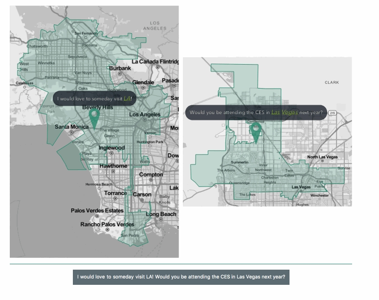
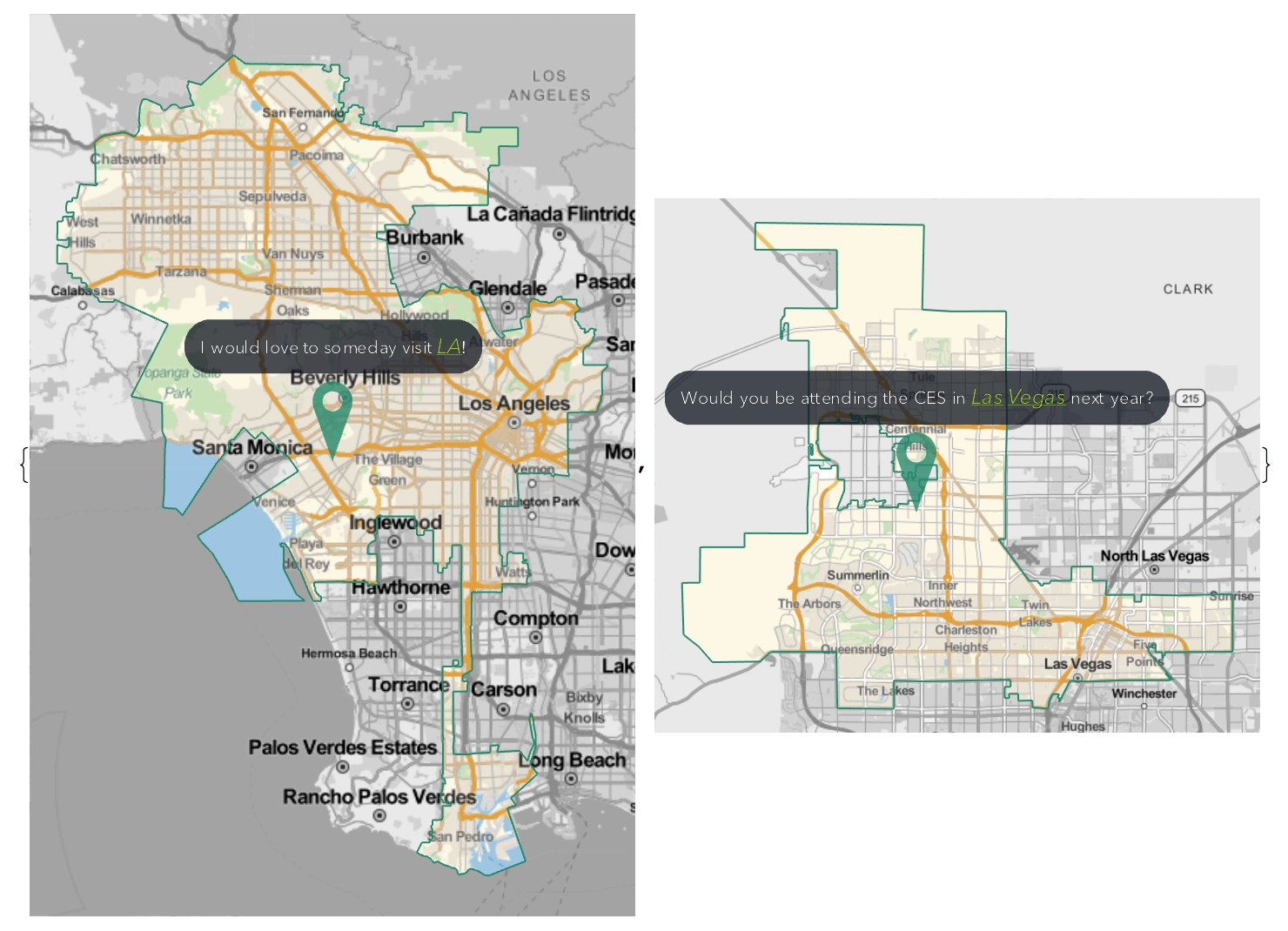
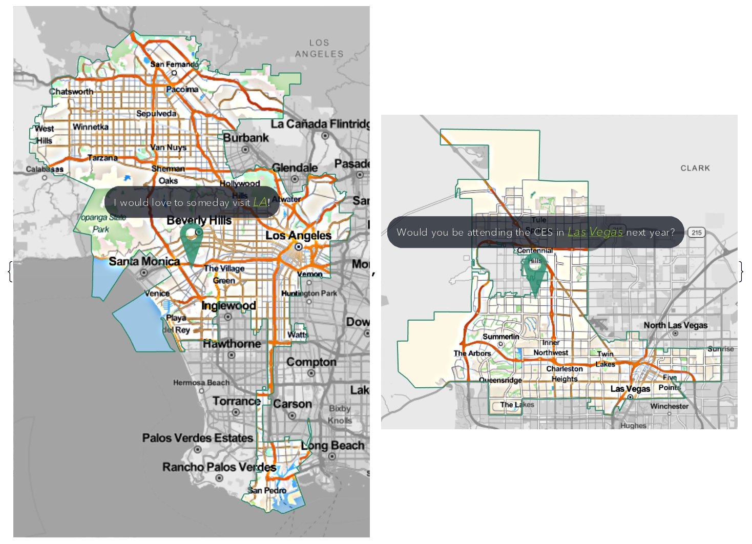
This produces a clean way of viewing the original text alongside the information (cities) extracted from it. We can style the maps in so many different ways. Here are a few:
1map2 = ParallelTable[2 Block[{city = cityNames[[c]], country = countryNames[[c]]},3 GeoGraphics[{GeoStyling["StreetMap"],4 EdgeForm[{col1, Thin, Opacity[1]}], Polygon[city], GeoMarker[city, pins[[c]], "Alignment" -> Bottom, "Scale" -> Scaled[1]]}, GeoBackground -> GeoStyling["StreetMap", GeoStylingImageFunction -> (ImageAdjust[ColorConvert[#1, "Grayscale"], {.5, -.2}] &)], ImageSize -> Scaled[.3]] // Quiet], {c, Range@Length@extrCities}]
1map4 = ParallelTable[2 Block[{city = cityNames[[c]], country = countryNames[[c]]},3 GeoGraphics[{GeoStyling["StreetMap", EdgeForm[{Thin, col1}], GeoStylingImageFunction -> (Sharpen[#1, 10] &)], Polygon[city], GeoMarker[city, pins[[c]], "Alignment" -> Bottom, "Scale" -> Scaled[1]]}, GeoBackground -> GeoStyling["StreetMap", GeoStylingImageFunction -> (ImageAdjust[ColorConvert[#1, "Grayscale"], {.5, -.2}] &)], ImageSize -> Scaled[.3]] // Quiet], {c, Range@Length@extrCities}]
Combined Maps
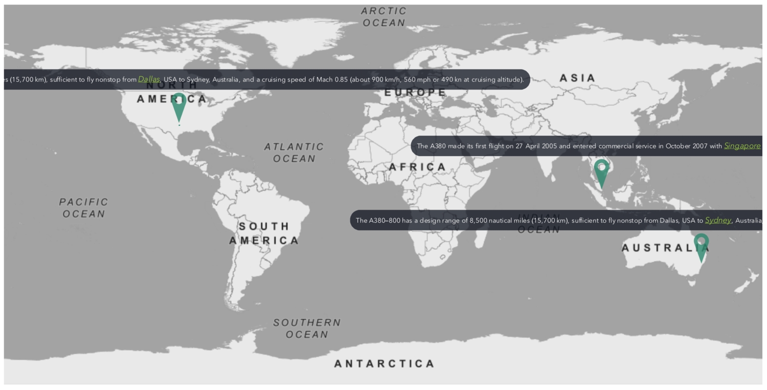
What if our original sentence contained, say, 10 different cities? In such a case, it'll be a lot more convenient to visualise all the cities on a single map; especially when there is a significant distance between the cities, this will be more insightful. This time, we'll use a larger piece of text, sourced from Wikipedia.
text = WikipediaData["Airbus A380", "SummaryPlaintext"]

If we evaluate the same code we previously used to extract the cities, we get the following result:

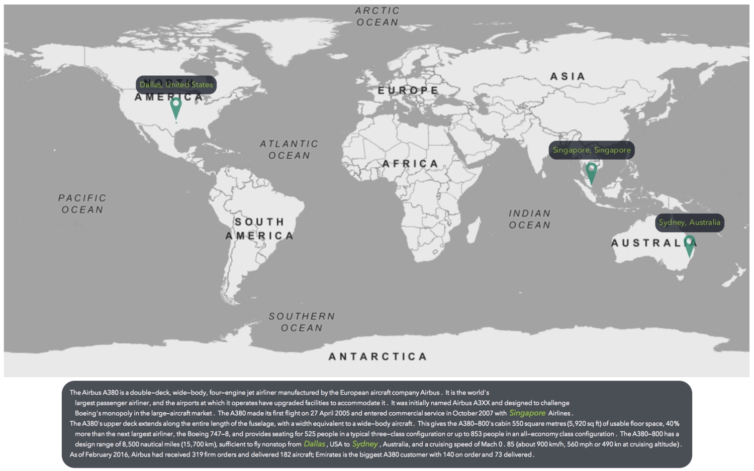
As you can see, this time, we have three cities on three different continents. So visualising them on individual maps will not give the bigger picture. Therefore, we'll combine them all into one larger map.
Our highlighted text will now contain all of the original text with the cities highlighted.
1thread = (extrCities[[#]] -> makeTooltip[extrCities[[#]], fullNames[[#]]])&/@Range@Length@extrCities;23textRow = Row[4 Style[#, White, FontFamily -> "Avenir Next", 10]&/@5 (StringSplit[text, Flatten@{" ", "." -> ".", "!" -> "!", "?" -> "?", thread}] /. thread)," " ,6Background -> Directive[ThemeColour, Opacity[.75]], FrameMargins -> 12, RoundingRadius -> 20, Frame -> True, FrameStyle -> None]

We will now modify our previous marker function to suit our new map.
1pinToMap2[highText2_] := Column[{2 Row[{3 Style[Row[highText2, ","], col2, FontFamily -> "Avenir Next", 12]4 }, Background -> Directive[ThemeColour, Opacity[.75]],5 FrameMargins -> 5, RoundingRadius -> 12, Frame -> True,6 FrameStyle -> None]7 ,8 Graphics[9 GraphicsGroup[{FaceForm[{col1, Opacity[.8]}],10 FilledCurve[{{Line[11 Join[{{0, 0}}, ({Cos[#1], 3 + Sin[#1]} &) /@12 Range[-((2 \[Pi])/20), \[Pi] + (2 \[Pi])/20, \[Pi]/13 20], {{0,14 0}}]]}, {Line[(0.5 {Cos[#1], 6 + Sin[#1]} &) /@15 Range[0, 2 \[Pi], \[Pi]/20]]}}]}], ImageSize -> 20]16 }, Alignment -> Center];1718pinToMap2[fullNames[[#]]]&/@Range@Length@extrCities

I came up with two different styles of visualising the combined map. The first style places the city marker (city, country) on the city, whilst the second style places the highlighted sentence on the city.
- Style 1
1style1 = Table[Block[{city = cityNames[[i]]}, {GeoStyling["StreetMap", EdgeForm[{Thin, col1}], GeoStylingImageFunction -> (ImageMultiply[Rasterize@ColorConvert[#1, "Grayscale"], Lighter[col1, .85]] &)],2 Polygon[city],GeoMarker[city, pinToMap2[fullNames[[i]]], "Alignment" -> Bottom,"Scale" -> Scaled[1]],city}]3 ,{i, Range@Length@extrCities}];
1Column[{2 GeoGraphics[style1, GeoBackground -> GeoStyling["StreetMap",3 GeoStylingImageFunction -> (ImageAdjust[ColorConvert[#1, "Grayscale"], {.5, -.2}] &)], ImageSize -> Full, GeoRange -> "World", GeoProjection -> Automatic],4 textRow5 }, Alignment -> Center]
- Style 2
1styles2 = Table[2 Block[{city = cityNames[[i]]},3 {GeoStyling["StreetMap", EdgeForm[{Thin, col1}], GeoStylingImageFunction -> (ImageMultiply[Rasterize@ColorConvert[#1, "Grayscale"], Lighter[col1, .85]] &)], Polygon[city], GeoMarker[city, pins[[i]], "Alignment" -> Bottom, "Scale" -> Scaled[1]], city}], {i, Range@Length@extrCities}];
1GeoGraphics[styles2,GeoBackground -> GeoStyling["StreetMap",2 GeoStylingImageFunction -> (ImageAdjust[ColorConvert[#1, "Grayscale"], {.5, -.2}] &)], ImageSize -> Full, GeoRange -> "World", GeoProjection -> Automatic3 ]
Conclusion
This article is the first part of a series on the analysis of textual data. It has shown how information extracted from a piece of text can be transformed into something useful. In this post, we looked at how one can extract the names of cities from a piece of text and visualise them on maps.
It doesn't end here. There are many other things you can do. For instance, you can also visualise current weather data and forecasts for the mentioned cities. Another example could be to find the shortest path (and distance) between the different cities.
In the next part of this series, more interesting and insightful analyses will be discussed. Stay tuned.
— MS