I was excited when I first heard about the Intel Edison when it was announced at the 2014 CES. At the time of this announcement, the Intel Edison was the size and shape of an SD card, yet running Linux, and had Wi-fi and Bluetooth onboard. What got me even more excited was that it was going to have Mathematica on it. An update revealed that a few changes were made to the Edison -- it was now bigger, had a different CPU and was more extensible. The Intel Edison now comes in three different forms:
- Intel Edison Compute Module -Intel Edison Kit for Arduino -Intel Edison Breakout Board Kit
I recently got the kit for Arduino and I've had so much fun playing around with it. In this post, you'll learn how to stream data from a temperature sensor and visualise it in Mathematica. You'll also see how easy automating data collection can be. There are so many helpful articles on Instructables that show how one can set up the Edison.
In addition to the Edison (for Arduino), other items you'll need are a Grove Base Shield and a Grove temperature sensor.
1. IoT Analytics Dashboard
The Intel IoT Analytics Dashboard allows one to manage connected devices, view charts of data from them, and do many other things. This tutorial shows you how to set it up.
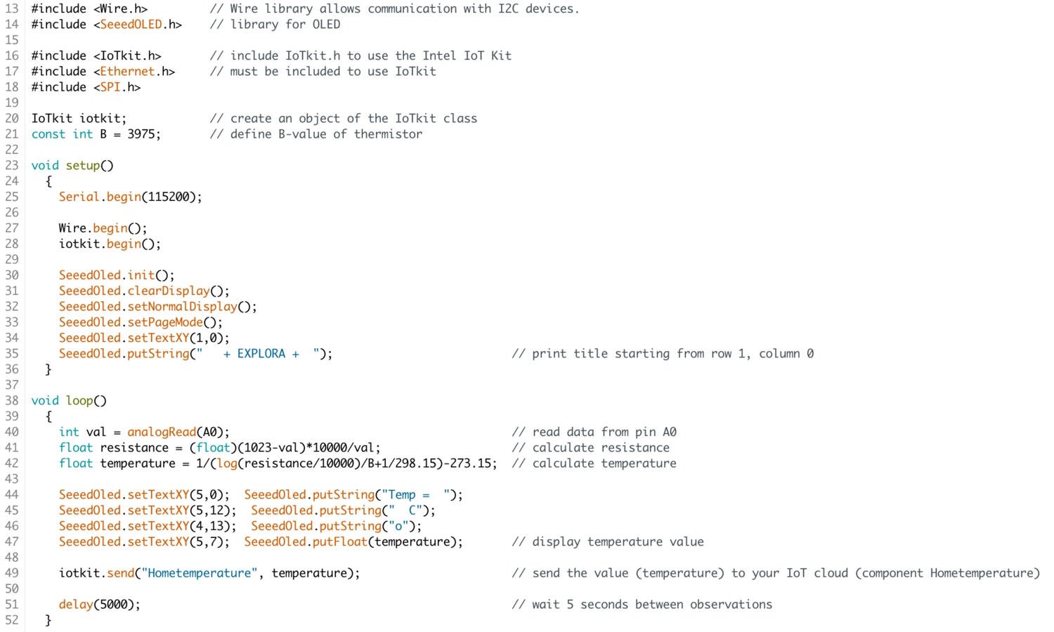
Once this is set up, you can begin sending data to the cloud. In this post, we'll send temperature data. Adapted from this sketch, the following Arduino code uploads temperature readings to the cloud once every five seconds. It also displays the current temperature on a 128x64 OLED. Within the same repository, you will find useful files and instructions on how to implement the IoT Analytics on Arduino.
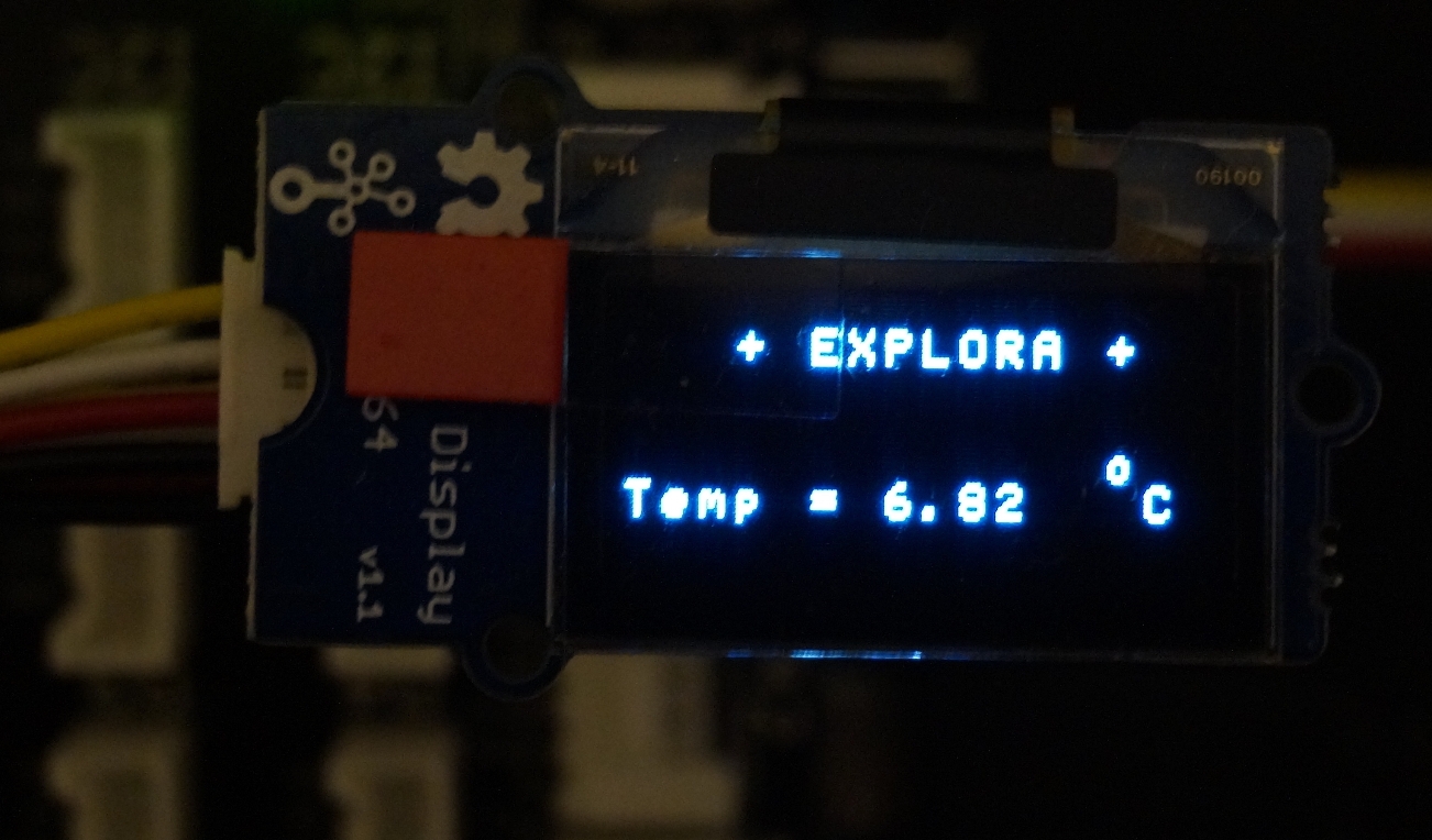
The OLED display looks like this:
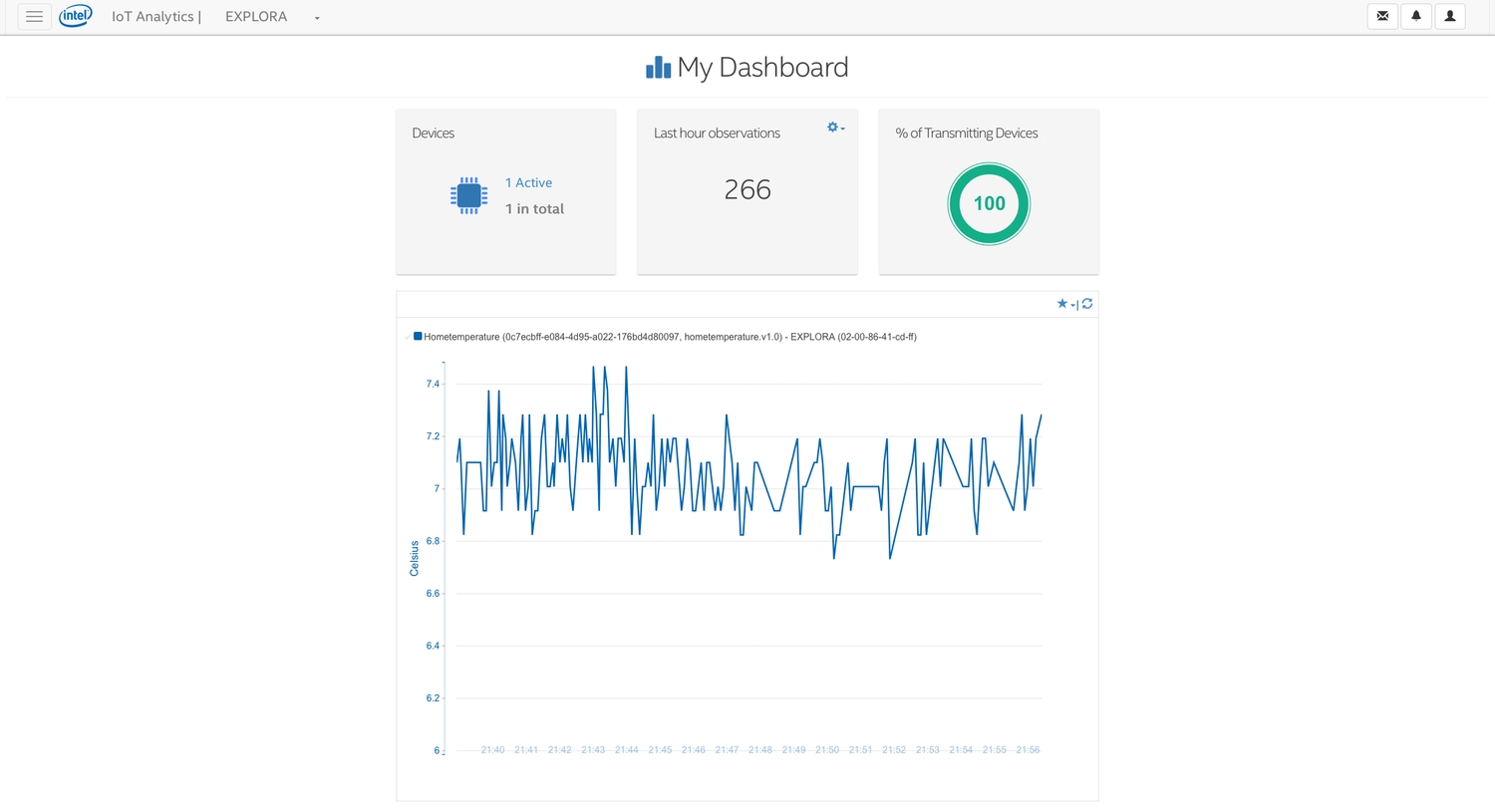
When signed in to the Intel Analytics Dashboard, you should see a summary of your devices, frequency of data upload, etc.
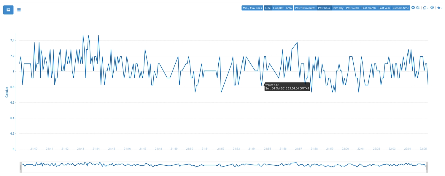
The Charts page shows a lot more detail on the selected device.
This article discusses, in great detail, the different aspects of the Intel Analytics website.
2. Arduino + Mathematica
2.1. Arduino Sketch
First, I uploaded this sketch to the Edison to record the temperature.
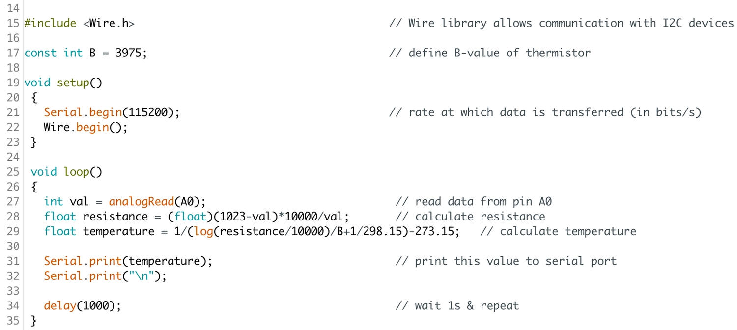
2.2. Connecting to Device
Given that I was using the Arduino kit, I initially thought it'd be befitting to open the device in Mathematica using the built-in Arduino library.
edison = DeviceOpen["Arduino", {"/dev/tty.usbmodem1413", "BaudRate" -> 115200}]
It appeared to have connected successfully but I couldn't read anything from, or write anything to the device. (I think this only works for the Arduino Uno.) I later turned to Serial after finding this post—which explains how to establish a serial connection to an accelerometer--on the Wolfram community, and it worked. :)
edison = DeviceOpen["Serial", {"/dev/tty.usbmodem1413", "BaudRate" -> 115200}]
So we've connected a device named edison over the serial port `/dev/tty.usbmodem1413 and we'll be transferring data at a rate of 115200 bits per second.
Warning: Ensure that the connection to the Edison on Mathematica is closed before uploading anything via the Arduino IDE or clicking the Serial Monitor button. Not doing this may halt the Arduino IDE.
2.3. Collecting Data
Following steps similar to the ones outlined in the post mentioned above, we can easily automate the collection of new data.
Let's create an empty list called data, to which we'll add every new reading as it comes in. This list will hold all of our data and values will be automatically added to it by task1, which is scheduled to do this every second.
1data = {};23task1 = RunScheduledTask[4 Block[{csv, raw},5 csv = FromCharacterCode[DeviceReadBuffer@edison]6 (* convert ASCII to normal characters *)7 raw = ImportString[csv, "List"];8 data = Join[data, raw];9 ], 110]
2.4. Visualising Data
We can now go ahead and visualise the data, in real-time. This can be done in several ways, we'll simply plot the temperature against time.

Plot 1 The first plot shows how the temperature varies over time (about two minutes), since we started collecting the data. That is, everything we've in data, up until now.

Plot 2 The second plot only shows data collected within the last minute. That is, the last 60 entries in data.

Remember that we're adding a new entry to the data every second, so this list will grow quickly. But memory-wise, the size of data should remain manageably small for playing around and trying things out. In fact, 2500 entries should amount to only about 60 Kb. However, allowing the plot to continually update itself for a long time will most likely result in a lot of memory being used. This can be checked using the MemoryInUse function.
3. Using Wolfram Data Drop
Instead of throwing everything into data, we can collect the temperature readings differently, using the Wolfram Data Drop. This way we can access, manipulate, and even add new entries to our databin - from wherever, at any time - in so many different ways including email and Twitter. We can swiftly gain insight into our data via Wolfram|Alpha. You can create a new databin either in Mathematica or online. Either way, you'll receive a short ID with which you can access it. For this section, I edited the Arduino code to send the data to the serial port every 5 seconds, rather than every second as before.
Let's create a new databin named TempDataBin, which stores temperature readings entered as temp.
1TempDataBin = CreateDataBin[{2 "Name" -> "TempDataBin",3 "Interpretation" -> "temp" -> Restricted["StructuredQuantity", "DegreesCelsius"]4}]
That creates a databin for us. Our databin short ID is 6FuSuRRs, and since this databin was created using a free account, it is only temporary and will expire a month from the creation date. Let's go ahead and add an entry to it--the most recent value stored in data.
DatabinAdd[TempDataBin, <|"temp" -> data[[-1]]|>]
And to view what we've just added:
Databin[TempDataBin, -1] // Values
<| temp -> {Quantity[8, "DegreesCelsius"]} |>
As you can see, our entry was automatically stored as a temperature reading, because that was what we defined all values of temp as when we created the databin.
Now we can go ahead and continuously add new data to this bin. To do this, we'll stop task1, and modify it to add to the bin as new data comes in.
1StopScheduledTask /@ ScheduledTasks[];2RemoveScheduledTask /@ ScheduledTasks[];34data2 = {};56task2 = RunScheduledTask[7 Block[{csv, raw},8 csv = FromCharacterCode[DeviceReadBuffer@edison];9 raw = ImportString[csv, "List"];10 data2 = Join[data2, raw];11 DatabinAdd[TempDataBin, <|"temp" -> data2[[-1]]|>];12 ], 7.513]
Similar to task1, task2 will add new data (the last value stored in data2) to our bin every 7.5 seconds, halfway between when that value was stored in data2 and when the next one will be.
After 60 entries have been added to the bin, an error occurs: "normal rate of 60 entries per hour exceeded." I assume this limitation only holds for a free account, but one can adjust the rate of adding new data to a bin to overcome this.
Anyway, let's view the entries that have been stored so far.
TimeSeries[TempDataBin] will show above gives us a summary of how and when the data was entered, while Values[TempDataBin] shows us all the entries in our databin.

Finally, DateListPlot[TempDataBin] shows us how the temperature varied over time.
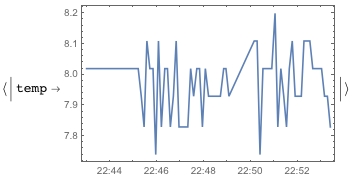
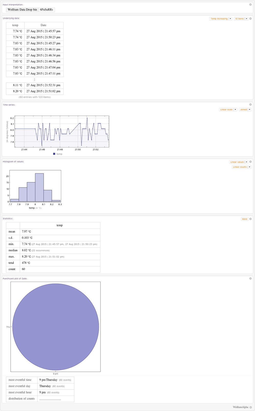
We can also view this in great detail, from anywhere, in Wolfram|Alpha. In Mathematica, this can be done by sending a WA request in the form of WolframAlpha["databin 6FuSuRRs"]. On the web computing "databin 6FuSuRRs" should result in something similar. You can download all your data as a .tsv file from the Data Drop website.
After a bit of fun (I hope) playing around with the Intel Edison, you can now disconnect it.
DeviceClose[edison]; Quit[];
In this post, we have seen how to:
- upload data to the Intel IoT Analytics Dashboard,
- collect and visualise data in real-time, in Mathematica, and
- store and visualise data using Wolfram Data Drop and Wolfram|Alpha.
Remember that we have used a relatively simple dataset, i.e., temperature values over time. For more complicated datasets, more extensive programming might be required.
— MS